Here we catalog the full set of Butcher tables included in ARKODE.
We group these into three categories: explicit, implicit and
additive. However, since the methods that comprise an additive
Runge–Kutta method are themselves explicit and implicit, their
component Butcher tables are listed within their separate
sections, but are referenced together in the additive section.
In each of the following tables, we use the following notation (shown
for a 3-stage method):
where here the method and embedding share stage \(A\) and
\(c\) values, but use their stages \(z_i\) differently through
the coefficients \(b\) and \(\tilde{b}\) to generate methods
of orders \(q\) (the main method) and \(p\) (the embedding,
typically \(q = p+1\), though sometimes this is reversed).
Method authors often use different naming conventions to categorize
their methods. For each of the methods below with an embedding, we follow the
uniform naming convention:
NAME-S-P-Q
where here
NAME is the author or the name provided by the author (if applicable),
S is the number of stages in the method,
P is the global order of accuracy for the embedding,
Q is the global order of accuracy for the method.
For methods without an embedding (e.g., fixed-step methods) P is omitted so
that methods follow the naming convention NAME-S-Q.
In the code, unique integer IDs are defined inside arkode_butcher_erk.h and
arkode_butcher_dirk.h for each method, which may be used by calling routines
to specify the desired method. These names are specified in fixedwidthfont at the start of each method’s section below.
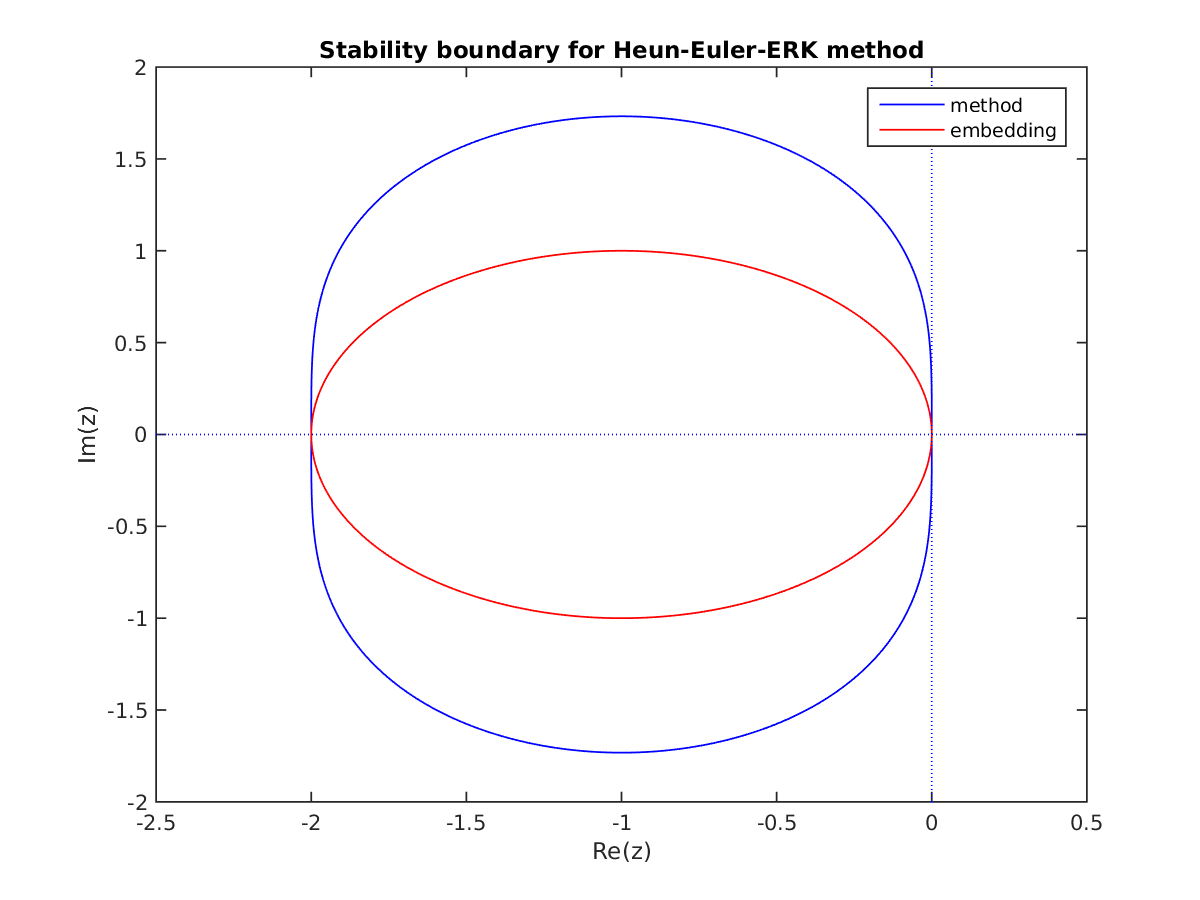
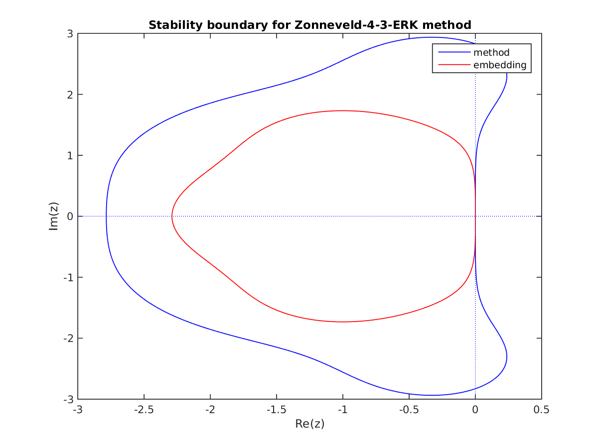
Additionally, for each method we provide a plot of the linear
stability region in the complex plane. These have been computed via
the following approach. For any Runge–Kutta method as defined above,
we may define the stability function
\[R(\eta) = 1 + \eta b [I - \eta A]^{-1} e,\]
where \(e\in\mathbb{R}^s\) is a column vector of all ones, \(\eta =
h\lambda\) and \(h\) is the time step size. If the stability
function satisfies \(|R(\eta)| \le 1\) for all eigenvalues,
\(\lambda\), of \(\frac{\partial }{\partial y}f(t,y)\) for a
given IVP, then the method will be linearly stable for that problem
and step size. The stability region
is typically given by an enclosed region of the complex plane, so it
is standard to search for the border of that region in order to
understand the method. Since all complex numbers with unit magnitude
may be written as \(e^{i\theta}\) for some value of \(\theta\),
we perform the following algorithm to trace out this boundary.
Define an array of values Theta. Since we wish for a
smooth curve, and since we wish to trace out the entire boundary,
we choose 10,000 linearly-spaced points from 0 to \(16\pi\).
Since some angles will correspond to multiple locations on the
stability boundary, by going beyond \(2\pi\) we ensure that all
boundary locations are plotted, and by using such a fine
discretization the Newton method (next step) is more likely to
converge to the root closest to the previous boundary point,
ensuring a smooth plot.
For each value \(\theta \in\)Theta, we solve the nonlinear
equation
\[0 = f(\eta) = R(\eta) - e^{i\theta}\]
using a finite-difference Newton iteration, using tolerance
\(10^{-7}\), and differencing parameter
\(\sqrt{\varepsilon}\) (\(\approx 10^{-8}\)).
In this iteration, we use as initial guess the solution from the
previous value of \(\theta\), starting with an initial-initial
guess of \(\eta=0\) for \(\theta=0\).
We then plot the resulting \(\eta\) values that trace the
stability region boundary.
We note that for any stable IVP method, the value \(\eta_0 =
-\varepsilon + 0i\) is always within the stability region. So in each
of the following pictures, the interior of the stability region is the
connected region that includes \(\eta_0\). Resultingly, methods
whose linear stability boundary is located entirely in the right
half-plane indicate an A-stable method.
In the category of explicit Runge–Kutta methods, ARKODE includes
methods that have orders 2 through 6, with embeddings that are of
orders 1 through 5. Each of ARKODE’s explicit Butcher tables are
specified via a unique ID:
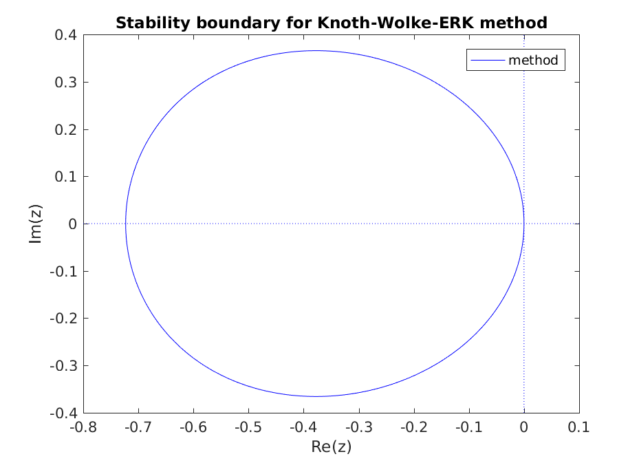
Accessible via the constant ARKODE_KNOTH_WOLKE_3_3 to
MRIStepSetMRITableNum() and ARKodeButcherTable_LoadERK().
This is the default 3th order slow and fast MRIStep method (from
[75]).
In the category of diagonally implicit Runge–Kutta methods, ARKODE
includes methods that have orders 2 through 5, with embeddings that are of
orders 1 through 4.
Each of ARKODE’s diagonally-implicit Butcher tables are
specified via a unique ID:
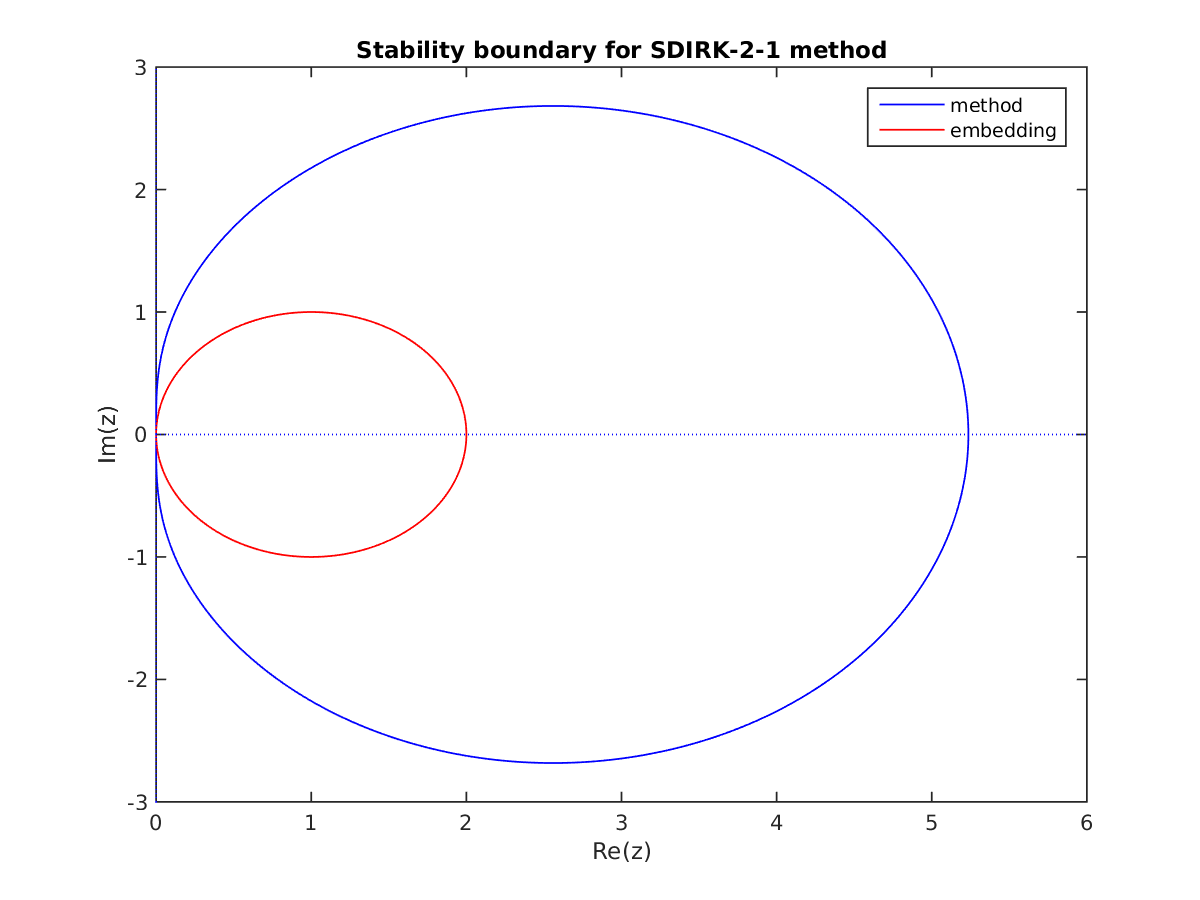
Accessible via the constant ARKODE_SDIRK_2_1_2 to
ARKStepSetTableNum() or
ARKodeButcherTable_LoadDIRK(). This is the default 2nd order
implicit method. Both the method and embedding are A- and B-stable.
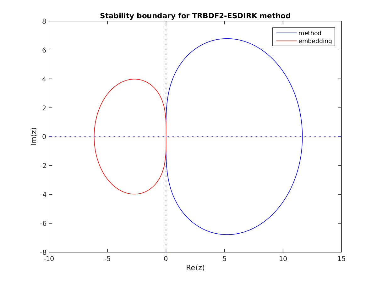
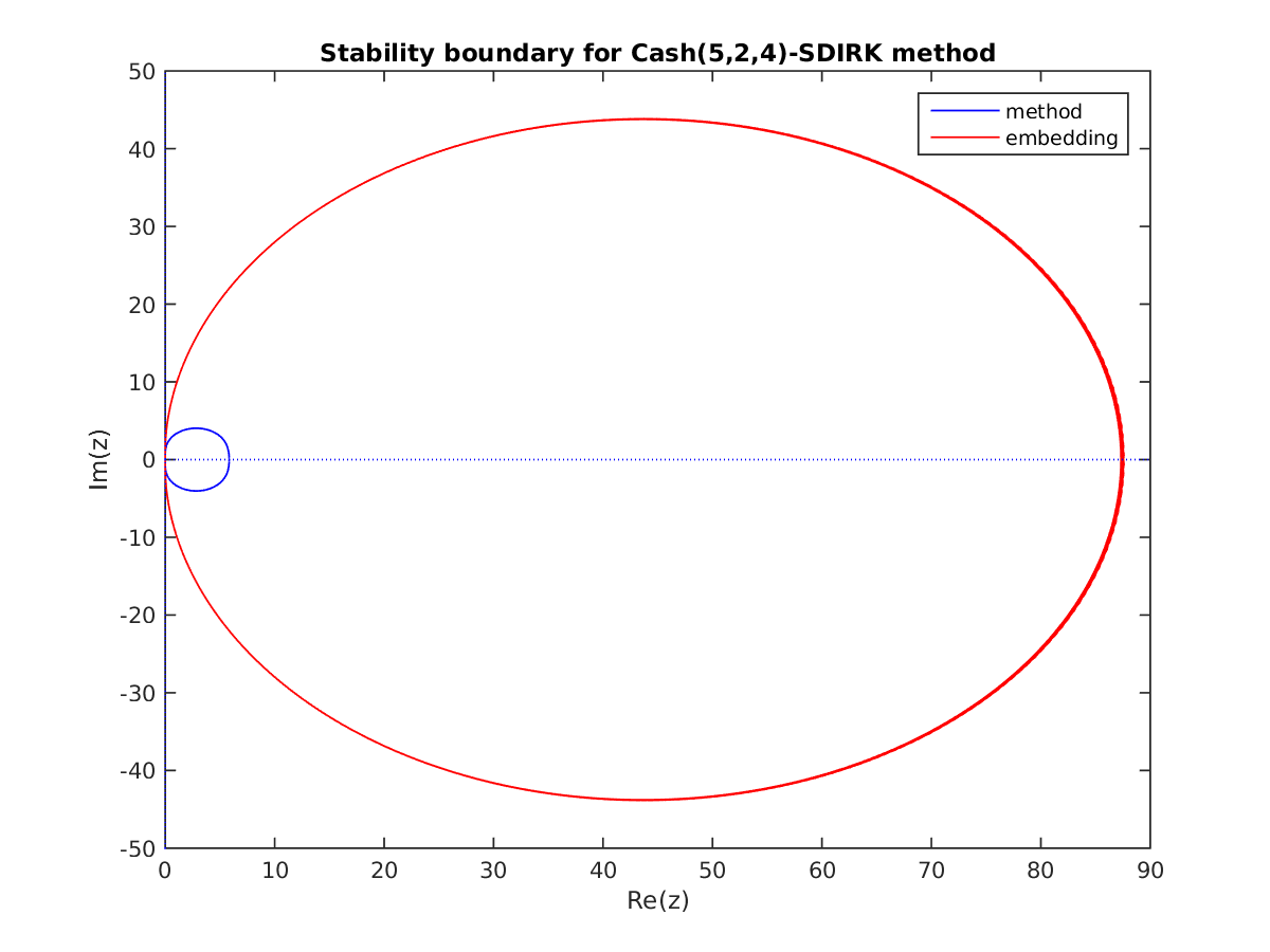
Accessible via the constant ARKODE_TRBDF2_3_3_2 to
ARKStepSetTableNum() or
ARKodeButcherTable_LoadDIRK(). As with Billington, here the
higher-order embedding is less stable than the lower-order method
(from [14]).
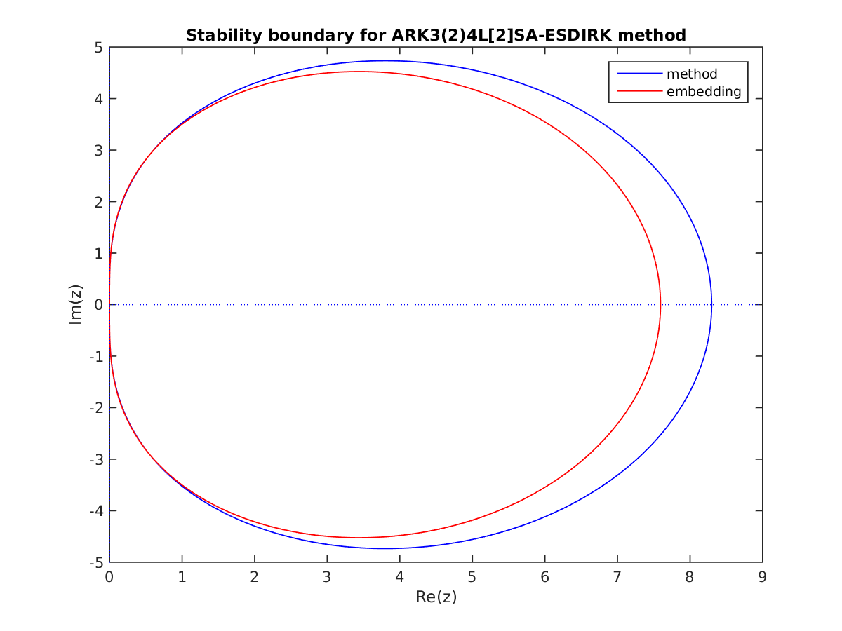
Accessible via the constant ARKODE_ARK324L2SA_DIRK_4_2_3 to
ARKStepSetTableNum() or
ARKodeButcherTable_LoadDIRK(). This is the default 3rd order
implicit method, and the implicit portion of the default 3rd order
additive method. Both the method and embedding are A-stable;
additionally the method is L-stable (this is the implicit portion of the
ARK3(2)4L[2]SA method from [71]).
Fig. 3.23 Linear stability region for the implicit ARK324L2SA-DIRK-4-2-3 method. The method’s
region is outlined in blue; the embedding’s region is in red.
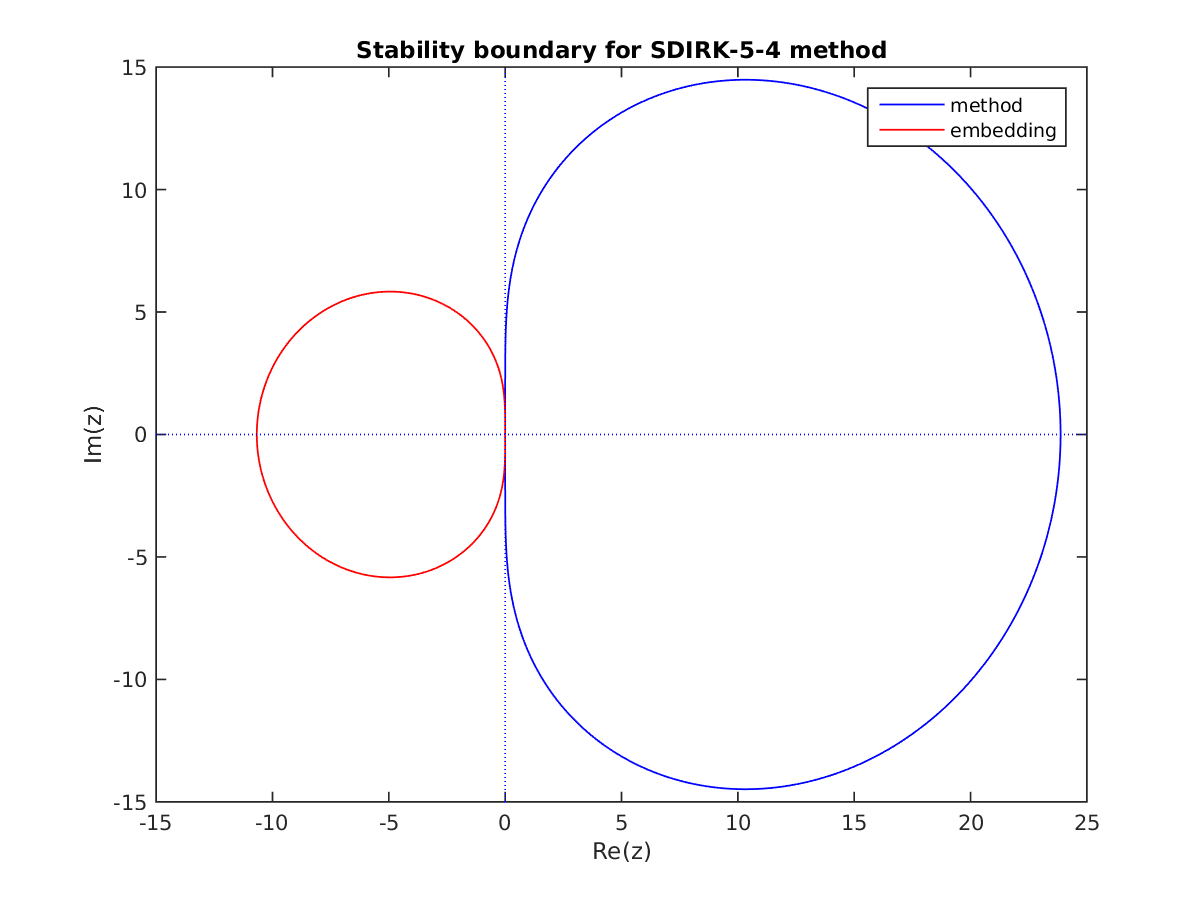
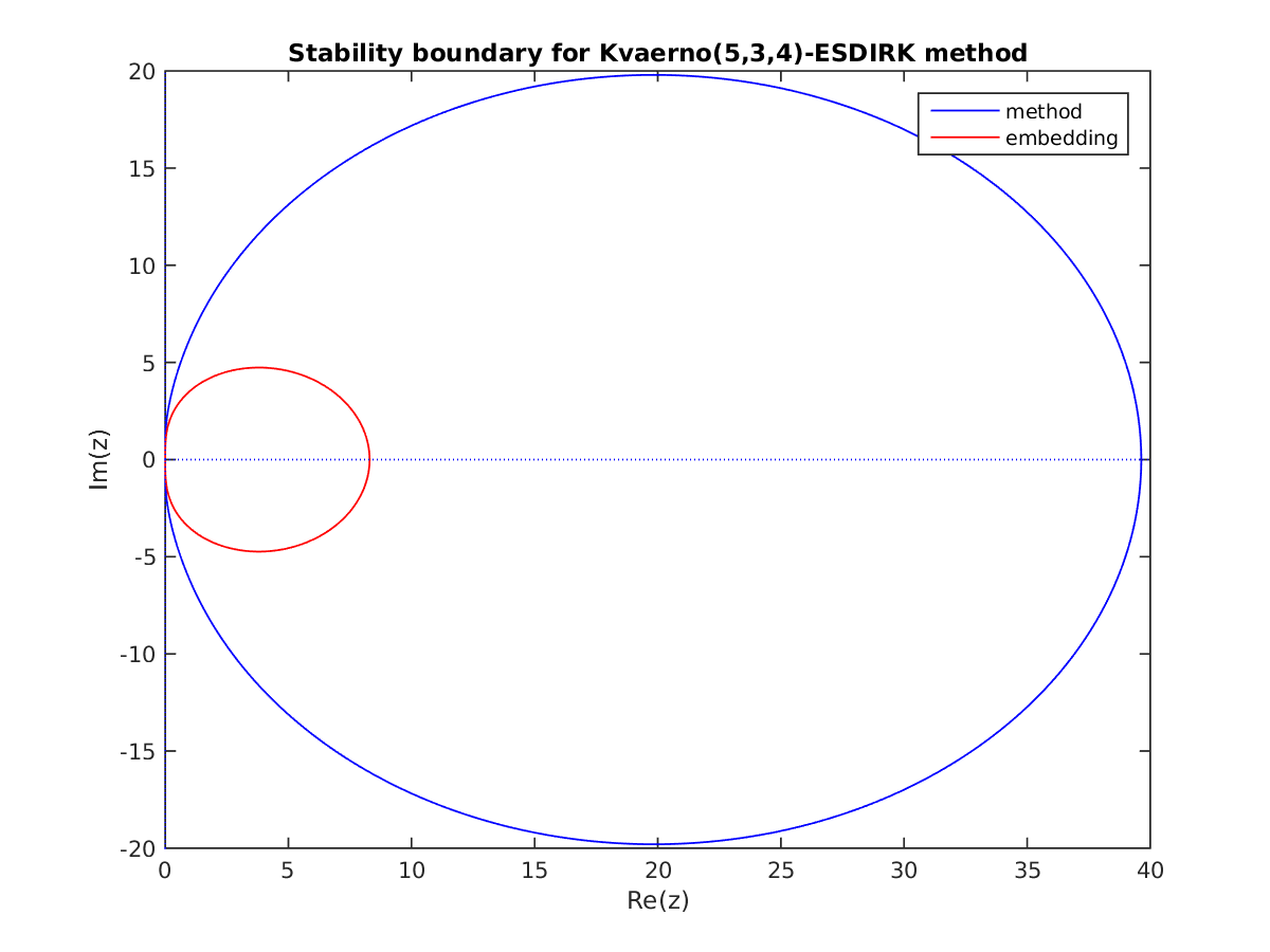
Accessible via the constant ARKODE_SDIRK_5_3_4 to
ARKStepSetTableNum() or
ARKodeButcherTable_LoadDIRK(). This is the default 4th order
implicit method. Here, the method is both A- and L-stable, although
the embedding has reduced stability (from [55]).
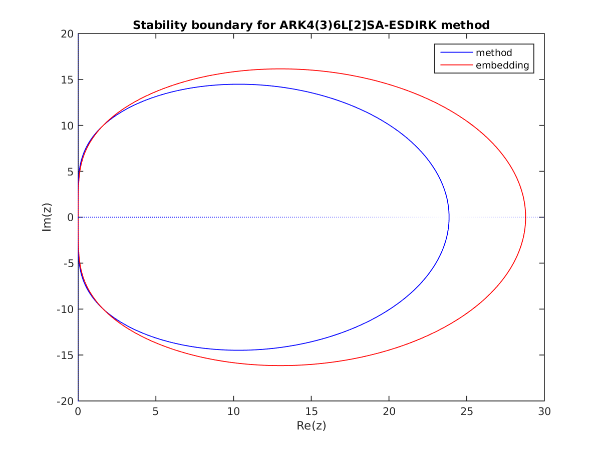
Accessible via the constant ARKODE_ARK436L2SA_DIRK_6_3_4 to
ARKStepSetTableNum() or
ARKodeButcherTable_LoadDIRK(). This is the implicit portion
of the default 4th order additive method. Both the method and
embedding are A-stable; additionally the method is L-stable (this is the
implicit portion of the ARK4(3)6L[2]SA method from [71]).
Accessible via the constant ARKODE_ARK437L2SA_DIRK_7_3_4 to
ARKStepSetTableNum() or
ARKodeButcherTable_LoadDIRK(). This is the implicit portion
of the 4th order ARK4(3)7L[2]SA method from [74].
Both the method and embedding are A- and L-stable.
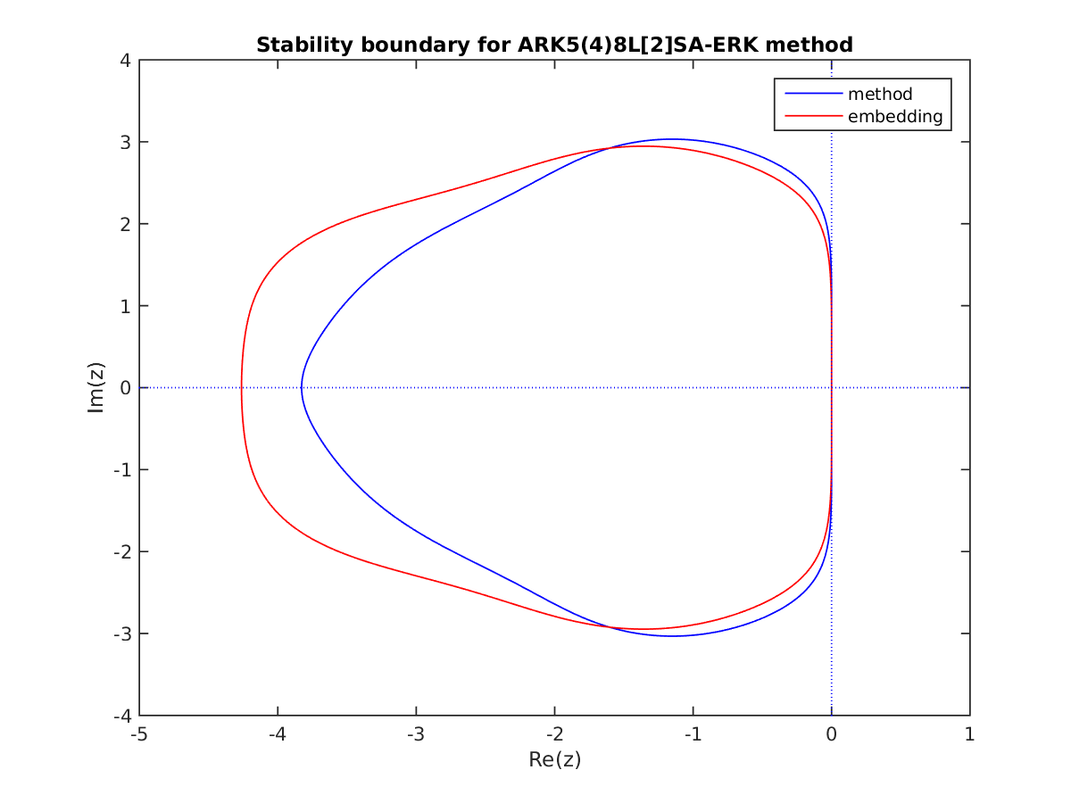
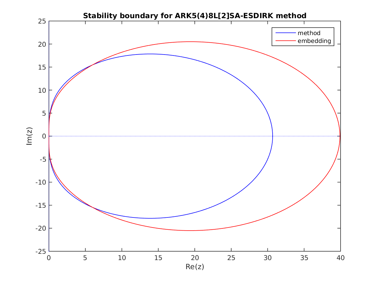
Accessible via the constant ARKODE_ARK548L2SA_DIRK_8_4_5 for
ARKStepSetTableNum() or
ARKodeButcherTable_LoadDIRK(). This is the default 5th order
implicit method, and the implicit portion of the default 5th order
additive method. Both the method and embedding are A-stable;
additionally the method is L-stable (the implicit portion of the ARK5(4)8L[2]SA
method from [71]).
Fig. 3.31 Linear stability region for the implicit ARK548L2SA-ESDIRK-8-4-5 method. The method’s
region is outlined in blue; the embedding’s region is in red.
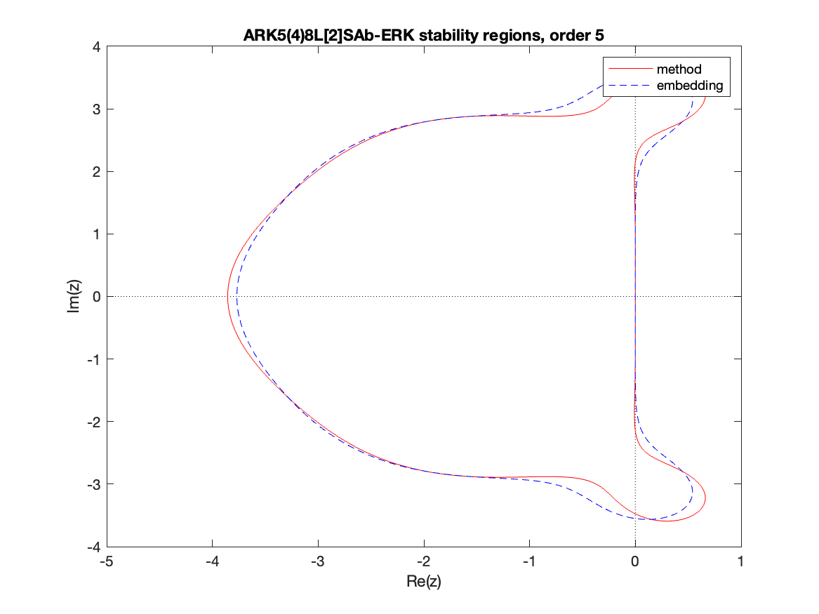
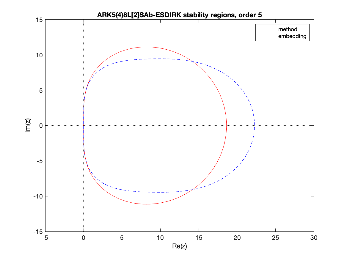
Accessible via the constant ARKODE_ARK548L2SAb_DIRK_8_4_5 for
ARKStepSetTableNum() or
ARKodeButcherTable_LoadDIRK(). Both the method and embedding are A-stable;
additionally the method is L-stable (this is the implicit portion of the 5th order
ARK5(4)8L[2]SA method from [74]).
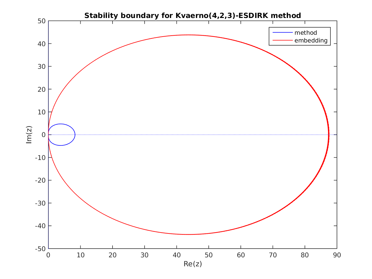
Accessible via the constant ARKODE_ESDIRK324L2SA_4_2_3 to
ARKStepSetTableNum() or ARKodeButcherTable_LoadDIRK().
This is the ESDIRK3(2)4L[2]SA method from [73].
Both the method and embedding are A- and L-stable.
Fig. 3.33 Linear stability region for the ESDIRK324L2SA-4-2-3 method method. The method’s
region is outlined in blue; the embedding’s region is in red.
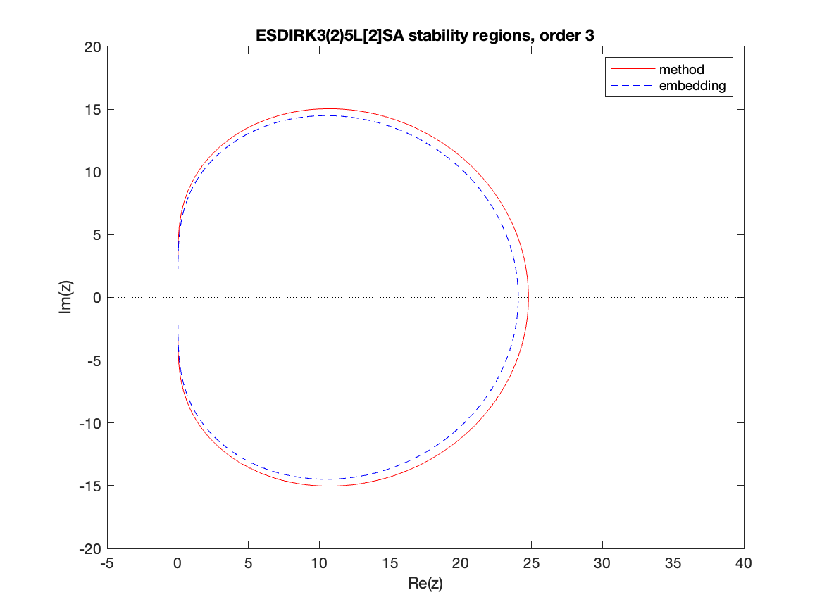
Accessible via the constant ARKODE_ESDIRK325L2SA_5_2_3 to
ARKStepSetTableNum() or ARKodeButcherTable_LoadDIRK().
This is the ESDIRK3(2)5L[2]SA method from [72].
Both the method and embedding are A- and L-stable.
Fig. 3.34 Linear stability region for the ESDIRK325L2SA-5-2-3 method method. The method’s
region is outlined in blue; the embedding’s region is in red.
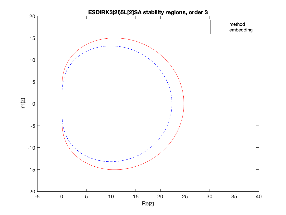
Accessible via the constant ARKODE_ESDIRK32I5L2SA_5_2_3 to
ARKStepSetTableNum() or ARKodeButcherTable_LoadDIRK().
This is the ESDIRK3(2I)5L[2]SA method from [72].
Both the method and embedding are A- and L-stable.
Fig. 3.35 Linear stability region for the ESDIRK32I5L2SA-5-2-3 method method. The method’s
region is outlined in blue; the embedding’s region is in red.
Accessible via the constant ARKODE_ESDIRK436L2SA_6_3_4 to
ARKStepSetTableNum() or ARKodeButcherTable_LoadDIRK().
This is the ESDIRK4(3)6L[2]SA method from [72].
Both the method and embedding are A- and L-stable.
Fig. 3.36 Linear stability region for the ESDIRK436L2SA-6-3-4 method method. The method’s
region is outlined in blue; the embedding’s region is in red.
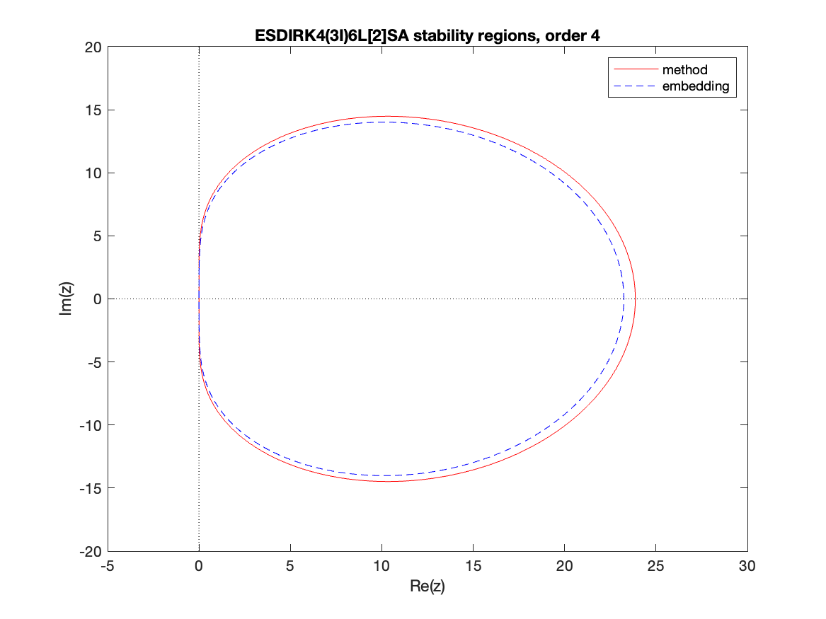
Accessible via the constant ARKODE_ESDIRK43I6L2SA_6_3_4 to
ARKStepSetTableNum() or ARKodeButcherTable_LoadDIRK().
This is the ESDIRK4(3I)6L[2]SA method from [72].
Both the method and embedding are A- and L-stable.
Fig. 3.37 Linear stability region for the ESDIRK43I6L2SA-6-3-4 method method. The method’s
region is outlined in blue; the embedding’s region is in red.
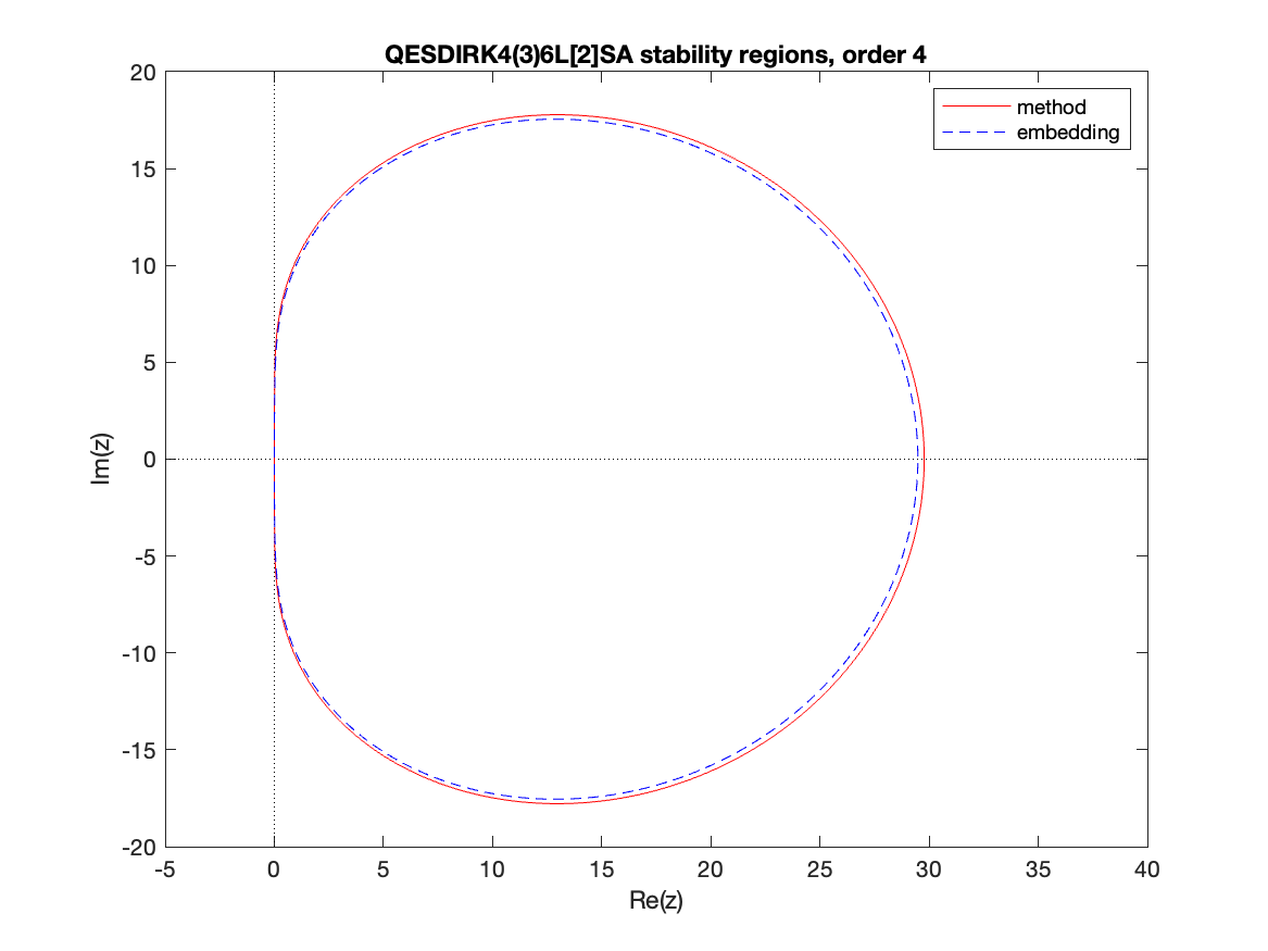
Accessible via the constant ARKODE_QESDIRK436L2SA_6_3_4 to
ARKStepSetTableNum() or ARKodeButcherTable_LoadDIRK().
This is the QESDIRK4(3)6L[2]SA method from [72].
Both the method and embedding are A- and L-stable.
Fig. 3.38 Linear stability region for the QESDIRK436L2SA-6-3-4 method method. The method’s
region is outlined in blue; the embedding’s region is in red.
Accessible via the constant ARKODE_ESDIRK437L2SA_7_3_4 to
ARKStepSetTableNum() or ARKodeButcherTable_LoadDIRK().
This is the ESDIRK4(3)7L[2]SA method from [73].
Both the method and embedding are A- and L-stable.
Fig. 3.39 Linear stability region for the ESDIRK437L2SA-7-3-4 method method. The method’s
region is outlined in blue; the embedding’s region is in red.
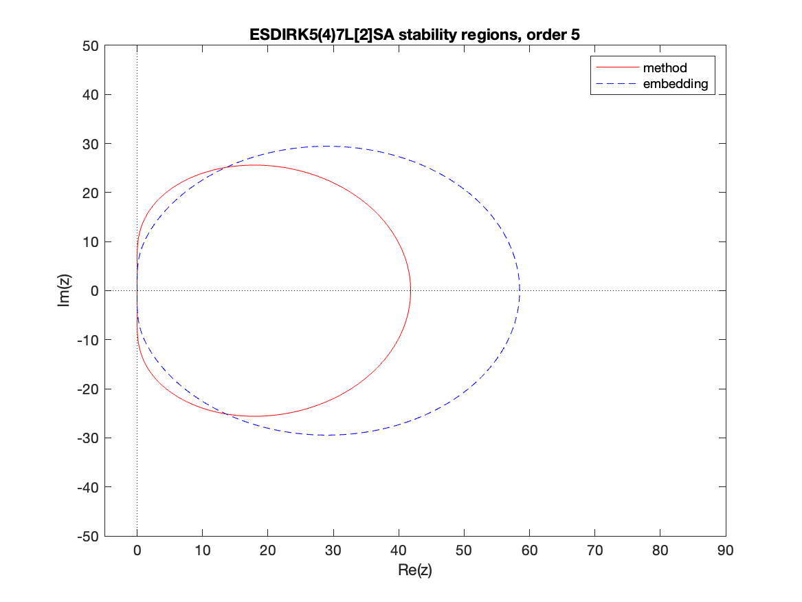
Accessible via the constant ARKODE_ESDIRK547L2SA_7_4_5 to
ARKStepSetTableNum() or ARKodeButcherTable_LoadDIRK().
This is the ESDIRK5(4)7L[2]SA method from [72].
Both the method and embedding are A- and L-stable.
Fig. 3.40 Linear stability region for the ESDIRK547L2SA-7-4-5 method method. The method’s
region is outlined in blue; the embedding’s region is in red.
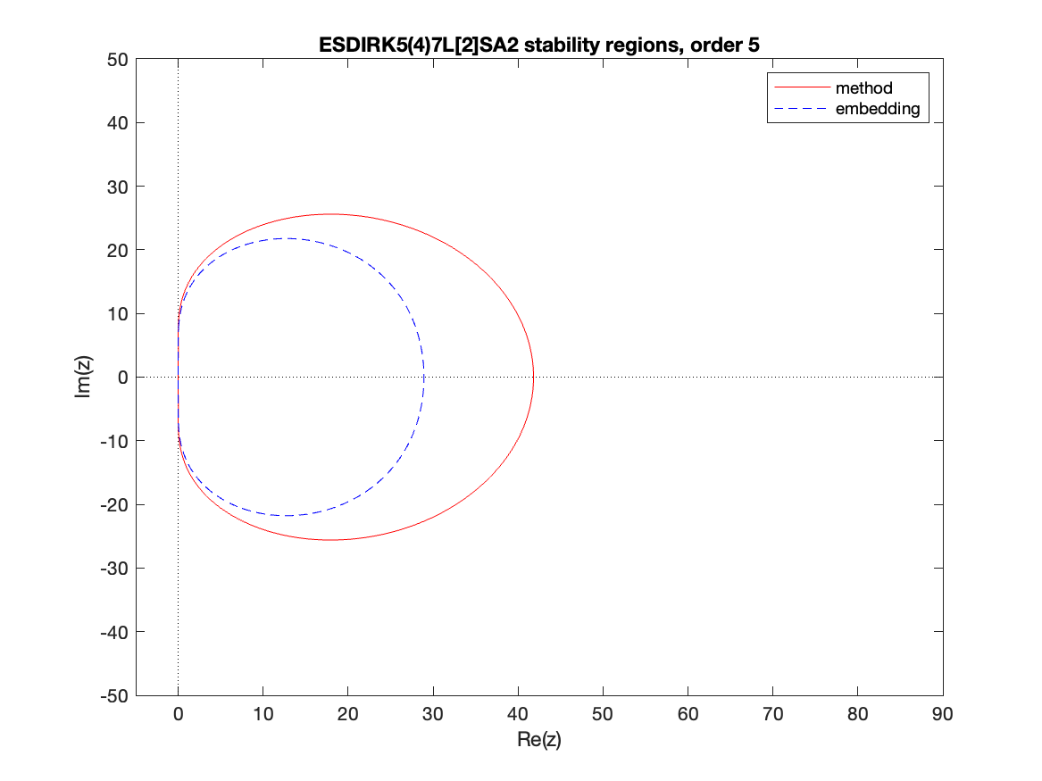
Accessible via the constant ARKODE_ESDIRK547L2SA2_7_4_5 to
ARKStepSetTableNum() or ARKodeButcherTable_LoadDIRK().
This is the ESDIRK5(4)7L[2]SA2 method from [73].
Both the method and embedding are A- and L-stable.
Fig. 3.41 Linear stability region for the ESDIRK547L2SA2-7-4-5 method method. The method’s
region is outlined in blue; the embedding’s region is in red.
In the category of additive Runge–Kutta methods for split implicit and
explicit calculations, ARKODE includes methods that have orders 3
through 5, with embeddings that are of orders 2 through 4. These
Butcher table pairs are as follows:
3rd-order pair:
§3.7.1.3 with §3.7.2.5,
corresponding to Butcher tables ARKODE_ARK324L2SA_ERK_4_2_3 and
ARKODE_ARK324L2SA_DIRK_4_2_3 for ARKStepSetTableNum().
4th-order pair:
§3.7.1.6 with §3.7.2.10,
corresponding to Butcher tables ARKODE_ARK436L2SA_ERK_6_3_4 and
ARKODE_ARK436L2SA_DIRK_6_3_4 for ARKStepSetTableNum().
4th-order pair:
§3.7.1.7 with §3.7.2.11,
corresponding to Butcher tables ARKODE_ARK437L2SA_ERK_7_3_4 and
ARKODE_ARK437L2SA_DIRK_7_3_4 for ARKStepSetTableNum().
5th-order pair:
§3.7.1.12 with §3.7.2.13,
corresponding to Butcher tables ARKODE_ARK548L2SA_ERK_8_4_5 and
ARKODE_ARK548L2SA_ERK_8_4_5 for ARKStepSetTableNum().
5th-order pair:
§3.7.1.13 with §3.7.2.14,
corresponding to Butcher tables ARKODE_ARK548L2SAb_ERK_8_4_5 and
ARKODE_ARK548L2SAb_ERK_8_4_5 for ARKStepSetTableNum().