4.2. Mathematical Considerations
CVODES solves ODE initial value problems (IVPs) in real \(N\)-space, which we write in the abstract form
where \(y \in \mathbb{R}^N\) and \(f: \mathbb{R} \times \mathbb{R}^N \rightarrow \mathbb{R}^N\). Here we use \(\dot{y}\) to denote \(\mathrm dy/\mathrm dt\). While we use \(t\) to denote the independent variable, and usually this is time, it certainly need not be. CVODES solves both stiff and nonstiff systems. Roughly speaking, stiffness is characterized by the presence of at least one rapidly damped mode, whose time constant is small compared to the time scale of the solution itself.
For problems (4.1) where the analytical solution \(y(t)\) satisfies an implicit constraint \(g(t,y)=0\) (including the initial condition, \(g(t_0,y_0)=0\)) for \(g(t,y): \mathbb{R} \times \mathbb{R}^N \rightarrow \mathbb{R}^{M}\) with \(M<N\), CVODES may be configured to explicitly enforce these constraints via solving the modified problem
Additionally, if (4.1) depends on some parameters \(p \in {\bf R}^{N_p}\), i.e.
CVODES can also compute first order derivative information, performing either forward sensitivity analysis or adjoint sensitivity analysis. In the first case, CVODES computes the sensitivities of the solution with respect to the parameters \(p\), while in the second case, CVODES computes the gradient of a derived function with respect to the parameters \(p\).
4.2.1. IVP solution
The methods used in CVODES are variable-order, variable-step multistep methods, based on formulas of the form
Here the \(y^n\) are computed approximations to \(y(t_n)\), and \(h_n = t_n - t_{n-1}\) is the step size. The user of CVODES must choose appropriately one of two multistep methods. For nonstiff problems, CVODES includes the Adams-Moulton formulas, characterized by \(K_1 = 1\) and \(K_2 = q-1\) above, where the order \(q\) varies between \(1\) and \(12\). For stiff problems, CVODES includes the Backward Differentiation Formulas (BDF) in so-called fixed-leading coefficient (FLC) form, given by \(K_1 = q\) and \(K_2 = 0\), with order \(q\) varying between \(1\) and \(5\). The coefficients are uniquely determined by the method type, its order, the recent history of the step sizes, and the normalization \(\alpha_{n,0} = -1\). See [32] and [91].
For either choice of formula, a nonlinear system must be solved (approximately) at each integration step. This nonlinear system can be formulated as either a rootfinding problem
or as a fixed-point problem
where \(a_n\equiv\sum_{i>0}(\alpha_{n,i}y^{n-i}+h_n\beta_{n,i} {\dot{y}}^{n-i})\).
In the process of controlling errors at various levels, CVODES uses a weighted root-mean-square norm, denoted \(|\cdot|_{\text{WRMS}}\), for all error-like quantities. The multiplicative weights used are based on the current solution and on the relative and absolute tolerances input by the user, namely
Because \(1/W_i\) represents a tolerance in the component \(y_i\), a vector whose norm is 1 is regarded as “small.” For brevity, we will usually drop the subscript WRMS on norms in what follows.
4.2.1.1. Nonlinear Solve
CVODES provides several nonlinear solver choices as well as the option of using a user-defined nonlinear solver (see §11). By default CVODES solves (4.5) with a Newton iteration which requires the solution of linear systems
in which
The exact variation of the Newton iteration depends on the choice of linear solver and is discussed below and in §11.7. For nonstiff systems, a fixed-point iteration (previously referred to as a functional iteration in this guide) solving (4.6) is also available. This involves evaluations of \(f\) only and can (optionally) use Anderson’s method [11, 58, 108, 166] to accelerate convergence (see §11.8 for more details). For any nonlinear solver, the initial guess for the iteration is a predicted value \(y^{n(0)}\) computed explicitly from the available history data.
For nonlinear solvers that require the solution of the linear system (4.8) (e.g., the default Newton iteration), CVODES provides several linear solver choices, including the option of a user-supplied linear solver module (see §10). The linear solver modules distributed with SUNDIALS are organized in two families, a direct family comprising direct linear solvers for dense, banded, or sparse matrices, and a spils family comprising scaled preconditioned iterative (Krylov) linear solvers. The methods offered through these modules are as follows:
dense direct solvers, including an internal implementation, an interface to BLAS/LAPACK, an interface to MAGMA [158] and an interface to the oneMKL library [3],
band direct solvers, including an internal implementation or an interface to BLAS/LAPACK,
sparse direct solver interfaces to various libraries, including KLU [4, 45], SuperLU_MT [9, 47, 105], SuperLU_Dist [8, 70, 106, 107], and cuSPARSE [7],
SPGMR, a scaled preconditioned GMRES (Generalized Minimal Residual method) solver,
SPFGMR, a scaled preconditioned FGMRES (Flexible Generalized Minimal Residual method) solver,
SPBCG, a scaled preconditioned Bi-CGStab (Bi-Conjugate Gradient Stable method) solver,
SPTFQMR, a scaled preconditioned TFQMR (Transpose-Free Quasi-Minimal Residual method) solver, or
PCG, a scaled preconditioned CG (Conjugate Gradient method) solver.
For large stiff systems, where direct methods are often not feasible, the combination of a BDF integrator and a preconditioned Krylov method yields a powerful tool because it combines established methods for stiff integration, nonlinear iteration, and Krylov (linear) iteration with a problem-specific treatment of the dominant source of stiffness, in the form of the user-supplied preconditioner matrix [26].
In addition, CVODES also provides a linear solver module which only uses a diagonal approximation of the Jacobian matrix.
In the case of a matrix-based linear solver, the default Newton iteration is a Modified Newton iteration, in that the iteration matrix \(M\) is fixed throughout the nonlinear iterations. However, in the case that a matrix-free iterative linear solver is used, the default Newton iteration is an Inexact Newton iteration, in which \(M\) is applied in a matrix-free manner, with matrix-vector products \(Jv\) obtained by either difference quotients or a user-supplied routine. With the default Newton iteration, the matrix \(M\) and preconditioner matrix \(P\) are updated as infrequently as possible to balance the high costs of matrix operations against other costs. Specifically, this matrix update occurs when:
starting the problem,
more than 20 steps have been taken since the last update,
the value \(\bar{\gamma}\) of \(\gamma\) at the last update satisfies \(|\gamma/\bar{\gamma} - 1| > 0.3\),
a non-fatal convergence failure just occurred, or
an error test failure just occurred.
When an update of \(M\) or \(P\) occurs, it may or may not involve a reevaluation of \(J\) (in \(M\)) or of Jacobian data (in \(P\)), depending on whether Jacobian error was the likely cause of the update. Reevaluating \(J\) (or instructing the user to update Jacobian data in \(P\)) occurs when:
starting the problem,
more than 50 steps have been taken since the last evaluation,
a convergence failure occurred with an outdated matrix, and the value \(\bar{\gamma}\) of \(\gamma\) at the last update satisfies \(|\gamma/\bar{\gamma} - 1| < 0.2\), or
a convergence failure occurred that forced a step size reduction.
The default stopping test for nonlinear solver iterations is related to the subsequent local error test, with the goal of keeping the nonlinear iteration errors from interfering with local error control. As described below, the final computed value \(y^{n(m)}\) will have to satisfy a local error test \(\|y^{n(m)} - y^{n(0)}\| \leq \epsilon\). Letting \(y^n\) denote the exact solution of (4.5), we want to ensure that the iteration error \(y^n - y^{n(m)}\) is small relative to \(\epsilon\), specifically that it is less than \(0.1 \epsilon\). (The safety factor \(0.1\) can be changed by the user.) For this, we also estimate the linear convergence rate constant \(R\) as follows. We initialize \(R\) to 1, and reset \(R = 1\) when \(M\) or \(P\) is updated. After computing a correction \(\delta_m = y^{n(m)}-y^{n(m-1)}\), we update \(R\) if \(m > 1\) as
Now we use the estimate
Therefore the convergence (stopping) test is
We allow at most 3 iterations (but this limit can be changed by the user). We also declare the iteration diverged if any \(\|\delta_m\| / \|\delta_{m-1}\| > 2\) with \(m > 1\). If convergence fails with \(J\) or \(P\) current, we are forced to reduce the step size, and we replace \(h_n\) by \(h_n = \eta_{\mathrm{cf}} * h_n\) where the default is \(\eta_{\mathrm{cf}} = 0.25\). The integration is halted after a preset number of convergence failures; the default value of this limit is 10, but this can be changed by the user.
When an iterative method is used to solve the linear system, its errors must also be controlled, and this also involves the local error test constant. The linear iteration error in the solution vector \(\delta_m\) is approximated by the preconditioned residual vector. Thus to ensure (or attempt to ensure) that the linear iteration errors do not interfere with the nonlinear error and local integration error controls, we require that the norm of the preconditioned residual be less than \(0.05 \cdot (0.1 \epsilon)\).
When the Jacobian is stored using either the SUNMATRIX_DENSE or SUNMATRIX_BAND matrix objects, the Jacobian may be supplied by a user routine, or approximated by difference quotients, at the user’s option. In the latter case, we use the usual approximation
The increments \(\sigma_j\) are given by
where \(U\) is the unit roundoff, \(\sigma_0\) is a dimensionless value, and \(W_j\) is the error weight defined in (4.7). In the dense case, this scheme requires \(N\) evaluations of \(f\), one for each column of \(J\). In the band case, the columns of \(J\) are computed in groups, by the Curtis-Powell-Reid algorithm, with the number of \(f\) evaluations equal to the bandwidth.
We note that with sparse and user-supplied SUNMatrix objects, the
Jacobian must be supplied by a user routine.
In the case of a Krylov method, preconditioning may be used on the left, on the right, or both, with user-supplied routines for the preconditioning setup and solve operations, and optionally also for the required matrix-vector products \(Jv\). If a routine for \(Jv\) is not supplied, these products are computed as
The increment \(\sigma\) is \(1/\|v\|\), so that \(\sigma v\) has norm 1.
4.2.1.2. Local Error Test
A critical part of CVODES — making it an ODE “solver” rather than just an ODE method, is its control of local error. At every step, the local error is estimated and required to satisfy tolerance conditions, and the step is redone with reduced step size whenever that error test fails. As with any linear multistep method, the local truncation error LTE, at order \(q\) and step size \(h\), satisfies an asymptotic relation
for some constant \(C\), under mild assumptions on the step sizes. A similar relation holds for the error in the predictor \(y^{n(0)}\). These are combined to get a relation
The local error test is simply \(|\mbox{LTE}| \leq 1\). Using the above, it is performed on the predictor-corrector difference \(\Delta_n \equiv y^{n(m)} - y^{n(0)}\) (with \(y^{n(m)}\) the final iterate computed), and takes the form
4.2.1.3. Step Size and Order Selection
If the local error test passes, the step is considered successful. If it fails, the step is rejected and a new step size \(h'\) is computed based on the asymptotic behavior of the local error, namely by the equation
Here 1/6 is a safety factor. A new attempt at the step is made, and the error test repeated. If it fails three times, the order \(q\) is reset to 1 (if \(q > 1\)), or the step is restarted from scratch (if \(q = 1\)). The ratio \(\eta = h'/h\) is limited above to \(\eta_{\mathrm{max\_ef}}\) (default 0.2) after two error test failures, and limited below to \(\eta_{\mathrm{min\_ef}}\) (default 0.1) after three. After seven failures, CVODES returns to the user with a give-up message.
In addition to adjusting the step size to meet the local error test, CVODES periodically adjusts the order, with the goal of maximizing the step size. The integration starts out at order 1 and varies the order dynamically after that. The basic idea is to pick the order \(q\) for which a polynomial of order \(q\) best fits the discrete data involved in the multistep method. However, if either a convergence failure or an error test failure occurred on the step just completed, no change in step size or order is done. At the current order \(q\), selecting a new step size is done exactly as when the error test fails, giving a tentative step size ratio
We consider changing order only after taking \(q+1\) steps at order \(q\), and then we consider only orders \(q' = q - 1\) (if \(q > 1\)) or \(q' = q + 1\) (if \(q < 5\)). The local truncation error at order \(q'\) is estimated using the history data. Then a tentative step size ratio is computed on the basis that this error, LTE\((q')\), behaves asymptotically as \(h^{q'+1}\). With safety factors of 1/6 and 1/10 respectively, these ratios are:
and
The new order and step size are then set according to
with \(q'\) set to the index achieving the above maximum. However, if we find that \(\eta < \eta_{\mathrm{max\_fx}}\) (default 1.5), we do not bother with the change. Also, \(\eta\) is always limited to \(\eta_{\mathrm{max\_gs}}\) (default 10), except on the first step, when it is limited to \(\eta_{\mathrm{max\_fs}} = 10^4\).
The various algorithmic features of CVODES described above, as inherited from VODE and VODPK, are documented in [25, 31, 83]. They are also summarized in [84].
Normally, CVODES takes steps until a user-defined output value \(t = t_{\text{out}}\) is overtaken, and then it computes \(y(t_{\text{out}})\) by interpolation. However, a “one step” mode option is available, where control returns to the calling program after each step. There are also options to force CVODES not to integrate past a given stopping point \(t = t_{\text{stop}}\).
4.2.1.4. Inequality Constraints
CVODES permits the user to impose optional inequality constraints on individual components of the solution vector \(y\). Any of the following four constraints can be imposed: \(y_i > 0\), \(y_i < 0\), \(y_i \geq 0\), or \(y_i \leq 0\). The constraint satisfaction is tested after a successful nonlinear system solution. If any constraint fails, we declare a convergence failure of the Newton iteration and reduce the step size. Rather than cutting the step size by some arbitrary factor, CVODES estimates a new step size \(h'\) using a linear approximation of the components in \(y\) that failed the constraint test (including a safety factor of \(0.9\) to cover the strict inequality case). If a step fails to satisfy the constraints repeatedly within a step attempt or fails with the minimum step size then the integration is halted and an error is returned. In this case the user may need to employ other strategies as discussed in §4.4.1.3.2 to satisfy the inequality constraints.
4.2.2. IVPs with constraints
For IVPs whose analytical solutions implicitly satisfy constraints as in (4.2), CVODES ensures that the solution satisfies the constraint equation by projecting a successfully computed time step onto the invariant manifold. As discussed in [53] and [140], this approach reduces the error in the solution and retains the order of convergence of the numerical method. Therefore, in an attempt to advance the solution to a new point in time (i.e., taking a new integration step), CVODES performs the following operations:
predict solution
solve nonlinear system and correct solution
project solution
test error
select order and step size for next step
and includes several recovery attempts in case there are convergence
failures (or difficulties) in the nonlinear solver or in the projection
step, or if the solution fails to satisfy the error test. Note that at
this time projection is only supported with BDF methods and the
projection function must be user-defined. See §4.4.1.3.8 and
CVodeSetProjFn() for more information on providing a
projection function to CVODE.
When using a coordinate projection method the solution \(y_n\) is obtained by projecting (orthogonally or otherwise) the solution \(\tilde{y}_n\) from step 2 above onto the manifold given by the constraint. As such \(y_n\) is computed as the solution of the nonlinear constrained least squares problem
The solution of (4.11) can be computed iteratively with a Newton method. Given an initial guess \(y_n^{(0)}\) the iterations are computed as
where the increment \(\delta y_n^{(i)}\) is the solution of the least-norm problem
where \(G(t,y) = \partial g(t,y) / \partial y\).
If the projected solution satisfies the error test then the step is accepted and the correction to the unprojected solution, \(\Delta_p = y_n - \tilde{y}_n\), is used to update the Nordsieck history array for the next step.
4.2.3. Preconditioning
When using a nonlinear solver that requires the solution of the linear system, e.g., the default Newton iteration (§11.7), CVODES makes repeated use of a linear solver to solve linear systems of the form \(M x = - r\), where \(x\) is a correction vector and \(r\) is a residual vector. If this linear system solve is done with one of the scaled preconditioned iterative linear solvers supplied with SUNDIALS, these solvers are rarely successful if used without preconditioning; it is generally necessary to precondition the system in order to obtain acceptable efficiency. A system \(A x = b\) can be preconditioned on the left, as \((P^{-1}A) x = P^{-1} b\); on the right, as \((A P^{-1}) P x = b\); or on both sides, as \((P_L^{-1} A P_R^{-1}) P_R x = P_L^{-1}b\). The Krylov method is then applied to a system with the matrix \(P^{-1}A\), or \(AP^{-1}\), or \(P_L^{-1} A P_R^{-1}\), instead of \(A\). In order to improve the convergence of the Krylov iteration, the preconditioner matrix \(P\), or the product \(P_L P_R\) in the last case, should in some sense approximate the system matrix \(A\). Yet at the same time, in order to be cost-effective, the matrix \(P\), or matrices \(P_L\) and \(P_R\), should be reasonably efficient to evaluate and solve. Finding a good point in this tradeoff between rapid convergence and low cost can be very difficult. Good choices are often problem-dependent (for example, see [26] for an extensive study of preconditioners for reaction-transport systems).
Most of the iterative linear solvers supplied with SUNDIALS allow for preconditioning either side, or on both sides, although we know of no situation where preconditioning on both sides is clearly superior to preconditioning on one side only (with the product \(P_L P_R\)). Moreover, for a given preconditioner matrix, the merits of left vs. right preconditioning are unclear in general, and the user should experiment with both choices. Performance will differ because the inverse of the left preconditioner is included in the linear system residual whose norm is being tested in the Krylov algorithm. As a rule, however, if the preconditioner is the product of two matrices, we recommend that preconditioning be done either on the left only or the right only, rather than using one factor on each side.
Typical preconditioners used with CVODES are based on approximations to the system Jacobian, \(J = \partial f / \partial y\). Since the matrix involved is \(M = I - \gamma J\), any approximation \(\bar{J}\) to \(J\) yields a matrix that is of potential use as a preconditioner, namely \(P = I - \gamma \bar{J}\). Because the Krylov iteration occurs within a nonlinear solver iteration and further also within a time integration, and since each of these iterations has its own test for convergence, the preconditioner may use a very crude approximation, as long as it captures the dominant numerical feature(s) of the system. We have found that the combination of a preconditioner with the Newton-Krylov iteration, using even a fairly poor approximation to the Jacobian, can be surprisingly superior to using the same matrix without Krylov acceleration (i.e., a modified Newton iteration), as well as to using the Newton-Krylov method with no preconditioning.
4.2.4. BDF stability limit detection
CVODES includes an algorithm, STALD (STAbility Limit Detection), which provides protection against potentially unstable behavior of the BDF multistep integration methods in certain situations, as described below.
When the BDF option is selected, CVODES uses Backward Differentiation Formula methods of orders 1 to 5. At order 1 or 2, the BDF method is A-stable, meaning that for any complex constant \(\lambda\) in the open left half-plane, the method is unconditionally stable (for any step size) for the standard scalar model problem \(\dot{y} = \lambda y\). For an ODE system, this means that, roughly speaking, as long as all modes in the system are stable, the method is also stable for any choice of step size, at least in the sense of a local linear stability analysis.
At orders 3 to 5, the BDF methods are not A-stable, although they are stiffly stable. In each case, in order for the method to be stable at step size \(h\) on the scalar model problem, the product \(h\lambda\) must lie within a region of absolute stability. That region excludes a portion of the left half-plane that is concentrated near the imaginary axis. The size of that region of instability grows as the order increases from 3 to 5. What this means is that, when running BDF at any of these orders, if an eigenvalue \(\lambda\) of the system lies close enough to the imaginary axis, the step sizes \(h\) for which the method is stable are limited (at least according to the linear stability theory) to a set that prevents \(h\lambda\) from leaving the stability region. The meaning of close enough depends on the order. At order 3, the unstable region is much narrower than at order 5, so the potential for unstable behavior grows with order.
System eigenvalues that are likely to run into this instability are ones that correspond to weakly damped oscillations. A pure undamped oscillation corresponds to an eigenvalue on the imaginary axis. Problems with modes of that kind call for different considerations, since the oscillation generally must be followed by the solver, and this requires step sizes (\(h \sim 1/\nu\), where \(\nu\) is the frequency) that are stable for BDF anyway. But for a weakly damped oscillatory mode, the oscillation in the solution is eventually damped to the noise level, and at that time it is important that the solver not be restricted to step sizes on the order of \(1/\nu\). It is in this situation that the new option may be of great value.
In terms of partial differential equations, the typical problems for which the stability limit detection option is appropriate are ODE systems resulting from semi-discretized PDEs (i.e., PDEs discretized in space) with advection and diffusion, but with advection dominating over diffusion. Diffusion alone produces pure decay modes, while advection tends to produce undamped oscillatory modes. A mix of the two with advection dominant will have weakly damped oscillatory modes.
The STALD algorithm attempts to detect, in a direct manner, the presence of a stability region boundary that is limiting the step sizes in the presence of a weakly damped oscillation [81]. The algorithm supplements (but differs greatly from) the existing algorithms in CVODES for choosing step size and order based on estimated local truncation errors. The STALD algorithm works directly with history data that is readily available in CVODES. If it concludes that the step size is in fact stability-limited, it dictates a reduction in the method order, regardless of the outcome of the error-based algorithm. The STALD algorithm has been tested in combination with the VODE solver on linear advection-dominated advection-diffusion problems [82], where it works well. The implementation in CVODES has been successfully tested on linear and nonlinear advection-diffusion problems, among others.
This stability limit detection option adds some computational overhead to the CVODES solution. (In timing tests, these overhead costs have ranged from 2% to 7% of the total, depending on the size and complexity of the problem, with lower relative costs for larger problems.) Therefore, it should be activated only when there is reasonable expectation of modes in the user’s system for which it is appropriate. In particular, if a CVODES solution with this option turned off appears to take an inordinately large number of steps at orders 3-5 for no apparent reason in terms of the solution time scale, then there is a good chance that step sizes are being limited by stability, and that turning on the option will improve the efficiency of the solution.
4.2.5. Rootfinding
The CVODES solver has been augmented to include a rootfinding feature. This means that, while integrating the Initial Value Problem (4.1), CVODES can also find the roots of a set of user-defined functions \(g_i(t,y)\) that depend both on \(t\) and on the solution vector \(y = y(t)\). The number of these root functions is arbitrary, and if more than one \(g_i\) is found to have a root in any given interval, the various root locations are found and reported in the order that they occur on the \(t\) axis, in the direction of integration.
Generally, this rootfinding feature finds only roots of odd multiplicity, corresponding to changes in sign of \(g_i(t,y(t))\), denoted \(g_i(t)\) for short. If a user root function has a root of even multiplicity (no sign change), it will probably be missed by CVODES. If such a root is desired, the user should reformulate the root function so that it changes sign at the desired root.
The basic scheme used is to check for sign changes of any \(g_i(t)\) over each time step taken, and then (when a sign change is found) to hone in on the root(s) with a modified secant method [79]. In addition, each time \(g\) is computed, CVODES checks to see if \(g_i(t) = 0\) exactly, and if so it reports this as a root. However, if an exact zero of any \(g_i\) is found at a point \(t\), CVODES computes \(g\) at \(t + \delta\) for a small increment \(\delta\), slightly further in the direction of integration, and if any \(g_i(t + \delta)=0\) also, CVODES stops and reports an error. This way, each time CVODES takes a time step, it is guaranteed that the values of all \(g_i\) are nonzero at some past value of \(t\), beyond which a search for roots is to be done.
At any given time in the course of the time-stepping, after suitable checking and adjusting has been done, CVODES has an interval \((t_{lo},t_{hi}]\) in which roots of the \(g_i(t)\) are to be sought, such that \(t_{hi}\) is further ahead in the direction of integration, and all \(g_i(t_{lo}) \neq 0\). The endpoint \(t_{hi}\) is either \(t_n\), the end of the time step last taken, or the next requested output time \(t_{\text{out}}\) if this comes sooner. The endpoint \(t_{lo}\) is either \(t_{n-1}\), the last output time \(t_{\text{out}}\) (if this occurred within the last step), or the last root location (if a root was just located within this step), possibly adjusted slightly toward \(t_n\) if an exact zero was found. The algorithm checks \(g_i\) at \(t_{hi}\) for zeros and for sign changes in \((t_{lo},t_{hi})\). If no sign changes were found, then either a root is reported (if some \(g_i(t_{hi}) = 0\)) or we proceed to the next time interval (starting at \(t_{hi}\)). If one or more sign changes were found, then a loop is entered to locate the root to within a rather tight tolerance, given by
Whenever sign changes are seen in two or more root functions, the one deemed most likely to have its root occur first is the one with the largest value of \(|g_i(t_{hi})|/|g_i(t_{hi}) - g_i(t_{lo})|\), corresponding to the closest to \(t_{lo}\) of the secant method values. At each pass through the loop, a new value \(t_{mid}\) is set, strictly within the search interval, and the values of \(g_i(t_{mid})\) are checked. Then either \(t_{lo}\) or \(t_{hi}\) is reset to \(t_{mid}\) according to which subinterval is found to include the sign change. If there is none in \((t_{lo},t_{mid})\) but some \(g_i(t_{mid}) = 0\), then that root is reported. The loop continues until \(|t_{hi}-t_{lo}| < \tau\), and then the reported root location is \(t_{hi}\).
In the loop to locate the root of \(g_i(t)\), the formula for \(t_{mid}\) is
where \(\alpha\) is a weight parameter. On the first two passes through the loop, \(\alpha\) is set to \(1\), making \(t_{mid}\) the secant method value. Thereafter, \(\alpha\) is reset according to the side of the subinterval (low vs. high, i.e., toward \(t_{lo}\) vs. toward \(t_{hi}\)) in which the sign change was found in the previous two passes. If the two sides were opposite, \(\alpha\) is set to 1. If the two sides were the same, \(\alpha\) is halved (if on the low side) or doubled (if on the high side). The value of \(t_{mid}\) is closer to \(t_{lo}\) when \(\alpha < 1\) and closer to \(t_{hi}\) when \(\alpha > 1\). If the above value of \(t_{mid}\) is within \(\tau/2\) of \(t_{lo}\) or \(t_{hi}\), it is adjusted inward, such that its fractional distance from the endpoint (relative to the interval size) is between .1 and .5 (.5 being the midpoint), and the actual distance from the endpoint is at least \(\tau/2\).
4.2.6. Pure Quadrature Integration
In many applications, and most notably during the backward integration phase of an adjoint sensitivity analysis run (see §4.2.8) it is of interest to compute integral quantities of the form
The most effective approach to compute \(z(t)\) is to extend the original problem with the additional ODEs (obtained by applying Leibnitz’s differentiation rule):
Note that this is equivalent to using a quadrature method based on the underlying linear multistep polynomial representation for \(y(t)\).
This can be done at the “user level” by simply exposing to CVODES the extended ODE system (4.3) + (4.13). However, in the context of an implicit integration solver, this approach is not desirable since the nonlinear solver module will require the Jacobian (or Jacobian-vector product) of this extended ODE. Moreover, since the additional states \(z\) do not enter the right-hand side of the ODE (4.13) and therefore the right-hand side of the extended ODE system, it is much more efficient to treat the ODE system (4.13) separately from the original system (4.3) by “taking out” the additional states \(z\) from the nonlinear system (4.5) that must be solved in the correction step of the LMM. Instead, “corrected” values \(z^n\) are computed explicitly as
once the new approximation \(y^n\) is available.
The quadrature variables \(z\) can be optionally included in the error test, in which case corresponding relative and absolute tolerances must be provided.
4.2.7. Forward Sensitivity Analysis
Typically, the governing equations of complex, large-scale models depend on various parameters, through the right-hand side vector and/or through the vector of initial conditions, as in (4.3). In addition to numerically solving the ODEs, it may be desirable to determine the sensitivity of the results with respect to the model parameters. Such sensitivity information can be used to estimate which parameters are most influential in affecting the behavior of the simulation or to evaluate optimization gradients (in the setting of dynamic optimization, parameter estimation, optimal control, etc.).
The solution sensitivity with respect to the model parameter \(p_i\) is defined as the vector \(s_i (t) = {\partial y(t)}/{\partial p_i}\) and satisfies the following forward sensitivity equations (or sensitivity equations for short):
obtained by applying the chain rule of differentiation to the original ODEs (4.3).
When performing forward sensitivity analysis, CVODES carries out the time integration of the combined system, (4.3) and (4.14), by viewing it as an ODE system of size \(N(N_s+1)\), where \(N_s\) is the number of model parameters \(p_i\), with respect to which sensitivities are desired (\(N_s \le N_p\)). However, major improvements in efficiency can be made by taking advantage of the special form of the sensitivity equations as linearizations of the original ODEs. In particular, for stiff systems, for which CVODES employs a Newton iteration, the original ODE system and all sensitivity systems share the same Jacobian matrix, and therefore the same iteration matrix \(M\) in (4.9).
The sensitivity equations are solved with the same linear multistep formula that was selected for the original ODEs and, if Newton iteration was selected, the same linear solver is used in the correction phase for both state and sensitivity variables. In addition, CVODES offers the option of including (full error control) or excluding (partial error control) the sensitivity variables from the local error test.
4.2.7.1. Forward sensitivity methods
In what follows we briefly describe three methods that have been proposed for the solution of the combined ODE and sensitivity system for the vector \({\hat y} = [y, s_1, \ldots , s_{N_s}]\).
Staggered Direct
In this approach [37], the nonlinear system (4.5) is first solved and, once an acceptable numerical solution is obtained, the sensitivity variables at the new step are found by directly solving (4.14) after the (BDF or Adams) discretization is used to eliminate \({\dot s}_i\). Although the system matrix of the above linear system is based on exactly the same information as the matrix \(M\) in (4.9), it must be updated and factored at every step of the integration, in contrast to an evaluation of \(M\) which is updated only occasionally. For problems with many parameters (relative to the problem size), the staggered direct method can outperform the methods described below [104]. However, the computational cost associated with matrix updates and factorizations makes this method unattractive for problems with many more states than parameters (such as those arising from semidiscretization of PDEs) and is therefore not implemented in CVODES.
Simultaneous Corrector
In this method [110], the discretization is applied simultaneously to both the original equations (4.3) and the sensitivity systems (4.14) resulting in the following nonlinear system
\[{\hat F}({\hat y}_n) \equiv {\hat y}_n - h_n\beta_{n,0} {\hat f}(t_n,\,{\hat y}_n) - {\hat a}_n = 0 \, ,\]where \({\hat f} = [ f(t,y,p), \ldots, ({\partial f}/{\partial y})(t,y,p) s_i + ({\partial f}/{\partial p_i})(t,y,p), \ldots ]\), and \({\hat a}_n\) is comprised of the terms in the discretization that depend on the solution at previous integration steps. This combined nonlinear system can be solved using a modified Newton method as in (4.8) by solving the corrector equation
(4.15)\[{\hat M}[{\hat y}_{n(m+1)}-{\hat y}_{n(m)}]=-{\hat F}({\hat y}_{n(m)})\]at each iteration, where
\[\begin{split}{\hat M} = \begin{bmatrix} M & & & & \\ - \gamma J_1 & M & & & \\ - \gamma J_2 & 0 & M & & \\ \vdots & \vdots & \ddots & \ddots & \\ - \gamma J_{N_s} & 0 & \ldots & 0 & M \end{bmatrix} \, ,\end{split}\]\(M\) is defined as in (4.9), and \(J_i = \dfrac{\partial}{\partial y}\left[ \left(\dfrac{\partial f}{\partial y}\right) s_i + \left(\dfrac{\partial f}{\partial p_i}\right) \right]\). It can be shown that 2-step quadratic convergence can be retained by using only the block-diagonal portion of \({\hat M}\) in the corrector equation (4.15). This results in a decoupling that allows the reuse of \(M\) without additional matrix factorizations. However, the products \(\left(\dfrac{\partial f}{\partial y}\right)s_i\) and the vectors \(\dfrac{\partial f}{\partial p_i}\) must still be reevaluated at each step of the iterative process (4.15) to update the sensitivity portions of the residual \({\hat G}\).
Staggered corrector
In this approach [59], as in the staggered direct method, the nonlinear system (4.5) is solved first using the Newton iteration (4.8). Then a separate Newton iteration is used to solve the sensitivity system (4.14):
(4.16)\[\begin{split}\begin{gathered} M [s_{i}^{n(m+1)} - s_{i}^{n(m)}]= \\ - \left[ s_{i}^{n(m)} - \gamma \left( \dfrac{\partial f}{\partial y} (t_n , y^n, p) s_{i}^{n(m)} + \dfrac{\partial f}{\partial p_i} (t_n , y^n , p) \right) -a_{i,n} \right] \, , \end{gathered}\end{split}\]where \(a_{i,n}=\sum_{j>0}(\alpha_{n,j}s_{i}^{n-j}+h_n\beta_{n,j}{{\dot s}_i}^{n-j})\). In other words, a modified Newton iteration is used to solve a linear system. In this approach, the vectors \(({\partial f}/{\partial p_i})\) need be updated only once per integration step, after the state correction phase (4.8) has converged. Note also that Jacobian-related data can be reused at all iterations (4.16) to evaluate the products \(({\partial f}/{\partial y}) s_i\).
CVODES implements the simultaneous corrector method and two flavors of the staggered corrector method which differ only if the sensitivity variables are included in the error control test. In the full error control case, the first variant of the staggered corrector method requires the convergence of the iterations (4.16) for all \(N_s\) sensitivity systems and then performs the error test on the sensitivity variables. The second variant of the method will perform the error test for each sensitivity vector \(s_i, (i=1,2,\ldots,N_s\)) individually, as they pass the convergence test. Differences in performance between the two variants may therefore be noticed whenever one of the sensitivity vectors \(s_i\) fails a convergence or error test.
An important observation is that the staggered corrector method, combined with a Krylov linear solver, effectively results in a staggered direct method. Indeed, the Krylov solver requires only the action of the matrix \(M\) on a vector and this can be provided with the current Jacobian information. Therefore, the modified Newton procedure (4.16) will theoretically converge after one iteration.
4.2.7.2. Selection of the absolute tolerances for sensitivity variables
If the sensitivities are included in the error test, CVODES provides an automated estimation of absolute tolerances for the sensitivity variables based on the absolute tolerance for the corresponding state variable. The relative tolerance for sensitivity variables is set to be the same as for the state variables. The selection of absolute tolerances for the sensitivity variables is based on the observation that the sensitivity vector \(s_i\) will have units of \([y]/[p_i]\). With this, the absolute tolerance for the \(j\)-th component of the sensitivity vector \(s_i\) is set to \({\mbox{atol}_j}/{|{\bar p}_i|}\), where \(\mbox{atol}_j\) are the absolute tolerances for the state variables and \(\bar p\) is a vector of scaling factors that are dimensionally consistent with the model parameters \(p\) and give an indication of their order of magnitude. This choice of relative and absolute tolerances is equivalent to requiring that the weighted root-mean-square norm of the sensitivity vector \(s_i\) with weights based on \(s_i\) be the same as the weighted root-mean-square norm of the vector of scaled sensitivities \({\bar s}_i = |{\bar p}_i| s_i\) with weights based on the state variables (the scaled sensitivities \({\bar s}_i\) being dimensionally consistent with the state variables). However, this choice of tolerances for the \(s_i\) may be a poor one, and the user of CVODES can provide different values as an option.
4.2.7.3. Evaluation of the sensitivity right-hand side
There are several methods for evaluating the right-hand side of the sensitivity systems (4.14): analytic evaluation, automatic differentiation, complex-step approximation, and finite differences (or directional derivatives). CVODES provides all the software hooks for implementing interfaces to automatic differentiation (AD) or complex-step approximation; future versions will include a generic interface to AD-generated functions. At the present time, besides the option for analytical sensitivity right-hand sides (user-provided), CVODES can evaluate these quantities using various finite difference-based approximations to evaluate the terms \(({\partial f}/{\partial y}) s_i\) and \(({\partial f}/{\partial p_i})\), or using directional derivatives to evaluate \(\left[ ({\partial f}/{\partial y}) s_i + ({\partial f}/{\partial p_i}) \right]\). As is typical for finite differences, the proper choice of perturbations is a delicate matter. CVODES takes into account several problem-related features: the relative ODE error tolerance \(\mbox{rtol}\), the machine unit roundoff \(U\), the scale factor \({\bar p}_i\), and the weighted root-mean-square norm of the sensitivity vector \(s_i\).
Using central finite differences as an example, the two terms \(({\partial f}/{\partial y}) s_i\) and \({\partial f}/{\partial p_i}\) in the right-hand side of (4.14) can be evaluated either separately:
or simultaneously:
or by adaptively switching between (4.17) + (4.18) and (4.19), depending on the relative size of the finite difference increments \(\sigma_i\) and \(\sigma_y\). In the adaptive scheme, if \(\rho = \max(\sigma_i/\sigma_y,\sigma_y/\sigma_i)\), we use separate evaluations if \(\rho > \rho_{max}\) (an input value), and simultaneous evaluations otherwise.
These procedures for choosing the perturbations (\(\sigma_i\), \(\sigma_y\), \(\sigma\)) and switching between finite difference and directional derivative formulas have also been implemented for one-sided difference formulas. Forward finite differences can be applied to \(({\partial f}/{\partial y}) s_i\) and \({\partial f}/{\partial p_i}\) separately, or the single directional derivative formula
can be used. In CVODES, the default value of \(\rho_{max}=0\) indicates the use of the second-order centered directional derivative formula (4.19) exclusively. Otherwise, the magnitude of \(\rho_{max}\) and its sign (positive or negative) indicates whether this switching is done with regard to (centered or forward) finite differences, respectively.
4.2.7.4. Quadratures depending on forward sensitivities
If pure quadrature variables are also included in the problem definition (see §4.2.6), CVODES does not carry their sensitivities automatically. Instead, we provide a more general feature through which integrals depending on both the states \(y\) of (4.3) and the state sensitivities \(s_i\) of (4.14) can be evaluated. In other words, CVODES provides support for computing integrals of the form:
If the sensitivities of the quadrature variables \(z\) of (4.13) are desired, these can then be computed by using:
as integrands for \(\bar{z}\), where \(q_y\) and \(q_p\) are the partial derivatives of the integrand function \(q\) of (4.13).
As with the quadrature variables \(z\), the new variables \(\bar z\) are also excluded from any nonlinear solver phase and “corrected” values \(\bar z^n\) are obtained through explicit formulas.
4.2.8. Adjoint Sensitivity Analysis
In the forward sensitivity approach described in the previous section, obtaining sensitivities with respect to \(N_s\) parameters is roughly equivalent to solving an ODE system of size \((1+N_s) N\). This can become prohibitively expensive, especially for large-scale problems, if sensitivities with respect to many parameters are desired. In this situation, the adjoint sensitivity method is a very attractive alternative, provided that we do not need the solution sensitivities \(s_i\), but rather the gradients with respect to model parameters of a relatively few derived functionals of the solution. In other words, if \(y(t)\) is the solution of (4.3), we wish to evaluate the gradient \({\mathrm dG}/{\mathrm dp}\) of
or, alternatively, the gradient \({\mathrm dg}/{\mathrm dp}\) of the function \(g(t, y, p)\) at the final time \(T\). The function \(g\) must be smooth enough that \(\partial g / \partial y\) and \(\partial g / \partial p\) exist and are bounded.
In what follows, we only sketch the analysis for the sensitivity problem for both \(G\) and \(g\). For details on the derivation see [36]. Introducing a Lagrange multiplier \(\lambda\), we form the augmented objective function
where \(*\) denotes the conjugate transpose. The gradient of \(G\) with respect to \(p\) is
where subscripts on functions \(f\) or \(g\) are used to denote partial derivatives and \(s = [s_1,\ldots,s_{N_s}]\) is the matrix of solution sensitivities. Applying integration by parts to the term \(\lambda^* {\dot s}\), and by requiring that \(\lambda\) satisfy
the gradient of \(G\) with respect to \(p\) is nothing but
The gradient of \(g(T,y,p)\) with respect to \(p\) can be then obtained by using the Leibniz differentiation rule. Indeed, from (4.20),
and therefore, taking into account that \(dG/dp\) in (4.22) depends on \(T\) both through the upper integration limit and through \(\lambda\), and that \(\lambda(T) = 0\),
where \(\mu\) is the sensitivity of \(\lambda\) with respect to the final integration limit \(T\). Thus \(\mu\) satisfies the following equation, obtained by taking the total derivative with respect to \(T\) of (4.21):
The final condition on \(\mu(T)\) follows from \((\partial\lambda/\partial t) + (\partial\lambda/\partial T) = 0\) at \(T\), and therefore, \(\mu(T) = -{\dot\lambda}(T)\).
The first thing to notice about the adjoint system (4.21) is that there is no explicit specification of the parameters \(p\); this implies that, once the solution \(\lambda\) is found, the formula (4.22) can then be used to find the gradient of \(G\) with respect to any of the parameters \(p\). The same holds true for the system (4.24) and the formula (4.23) for gradients of \(g(T,y,p)\). The second important remark is that the adjoint systems (4.21) and (4.24) are terminal value problems which depend on the solution \(y(t)\) of the original IVP (4.3). Therefore, a procedure is needed for providing the states \(y\) obtained during a forward integration phase of (4.3) to CVODES during the backward integration phase of (4.21) or (4.24). The approach adopted in CVODES, based on checkpointing, is described below.
4.2.9. Checkpointing scheme
During the backward integration, the evaluation of the right-hand side of the adjoint system requires, at the current time, the states \(y\) which were computed during the forward integration phase. Since CVODES implements variable-step integration formulas, it is unlikely that the states will be available at the desired time and so some form of interpolation is needed. The CVODES implementation being also variable-order, it is possible that during the forward integration phase the order may be reduced as low as first order, which means that there may be points in time where only \(y\) and \({\dot y}\) are available. These requirements therefore limit the choices for possible interpolation schemes. CVODES implements two interpolation methods: a cubic Hermite interpolation algorithm and a variable-degree polynomial interpolation method which attempts to mimic the BDF interpolant for the forward integration.
However, especially for large-scale problems and long integration intervals, the number and size of the vectors \(y\) and \({\dot y}\) that would need to be stored make this approach computationally intractable. Thus, CVODES settles for a compromise between storage space and execution time by implementing a so-called checkpointing scheme. At the cost of at most one additional forward integration, this approach offers the best possible estimate of memory requirements for adjoint sensitivity analysis. To begin with, based on the problem size \(N\) and the available memory, the user decides on the number \(N_d\) of data pairs (\(y\), \({\dot y}\)) if cubic Hermite interpolation is selected, or on the number \(N_d\) of \(y\) vectors in the case of variable-degree polynomial interpolation, that can be kept in memory for the purpose of interpolation. Then, during the first forward integration stage, after every \(N_d\) integration steps a checkpoint is formed by saving enough information (either in memory or on disk) to allow for a hot restart, that is a restart which will exactly reproduce the forward integration. In order to avoid storing Jacobian-related data at each checkpoint, a reevaluation of the iteration matrix is forced before each checkpoint. At the end of this stage, we are left with \(N_c\) checkpoints, including one at \(t_0\). During the backward integration stage, the adjoint variables are integrated from \(T\) to \(t_0\) going from one checkpoint to the previous one. The backward integration from checkpoint \(i+1\) to checkpoint \(i\) is preceded by a forward integration from \(i\) to \(i+1\) during which the \(N_d\) vectors \(y\) (and, if necessary \({\dot y}\)) are generated and stored in memory for interpolation (see Fig. 4.1).
Note
The degree of the interpolation polynomial is always that of the current BDF order for the forward interpolation at the first point to the right of the time at which the interpolated value is sought (unless too close to the \(i\)-th checkpoint, in which case it uses the BDF order at the right-most relevant point). However, because of the FLC BDF implementation §4.2.1, the resulting interpolation polynomial is only an approximation to the underlying BDF interpolant.
The Hermite cubic interpolation option is present because it was implemented chronologically first and it is also used by other adjoint solvers (e.g. DASPKADJOINT. The variable-degree polynomial is more memory-efficient (it requires only half of the memory storage of the cubic Hermite interpolation) and is more accurate. The accuracy differences are minor when using BDF (since the maximum method order cannot exceed 5), but can be significant for the Adams method for which the order can reach 12.
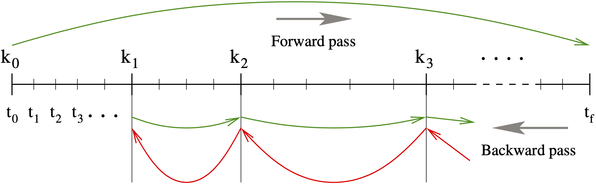
Fig. 4.1 Illustration of the checkpointing algorithm for generation of the forward solution during the integration of the adjoint system.
This approach transfers the uncertainty in the number of integration steps in the forward integration phase to uncertainty in the final number of checkpoints. However, \(N_c\) is much smaller than the number of steps taken during the forward integration, and there is no major penalty for writing/reading the checkpoint data to/from a temporary file. Note that, at the end of the first forward integration stage, interpolation data are available from the last checkpoint to the end of the interval of integration. If no checkpoints are necessary (\(N_d\) is larger than the number of integration steps taken in the solution of (4.3)), the total cost of an adjoint sensitivity computation can be as low as one forward plus one backward integration. In addition, CVODES provides the capability of reusing a set of checkpoints for multiple backward integrations, thus allowing for efficient computation of gradients of several functionals (4.20).
Finally, we note that the adjoint sensitivity module in CVODES provides the necessary infrastructure to integrate backwards in time any ODE terminal value problem dependent on the solution of the IVP (4.3), including adjoint systems (4.21) or (4.24), as well as any other quadrature ODEs that may be needed in evaluating the integrals in (4.22) or (4.23). In particular, for ODE systems arising from semi-discretization of time-dependent PDEs, this feature allows for integration of either the discretized adjoint PDE system or the adjoint of the discretized PDE.
4.2.10. Second-order sensitivity analysis
In some applications (e.g., dynamically-constrained optimization) it may be desirable to compute second-order derivative information. Considering the ODE problem (4.3) and some model output functional, \(g(y)\) then the Hessian \(d^2g/dp^2\) can be obtained in a forward sensitivity analysis setting as
where \(\otimes\) is the Kronecker product. The second-order sensitivities are solution of the matrix ODE system:
where \(y_p\) is the first-order sensitivity matrix, the solution of \(N_p\) systems (4.14), and \(y_{pp}\) is a third-order tensor. It is easy to see that, except for situations in which the number of parameters \(N_p\) is very small, the computational cost of this so-called forward-over-forward approach is exorbitant as it requires the solution of \(N_p + N_p^2\) additional ODE systems of the same dimension \(N\) as (4.3).
Note
For the sake of simplifity in presentation, we do not include explicit dependencies of \(g\) on time \(t\) or parameters \(p\). Moreover, we only consider the case in which the dependency of the original ODE (4.3) on the parameters \(p\) is through its initial conditions only. For details on the derivation in the general case, see [115].
A much more efficient alternative is to compute Hessian-vector products using a so-called forward-over-adjoint approach. This method is based on using the same “trick” as the one used in computing gradients of pointwise functionals with the adjoint method, namely applying a formal directional forward derivation to one of the gradients of (4.22) or (4.23). With that, the cost of computing a full Hessian is roughly equivalent to the cost of computing the gradient with forward sensitivity analysis. However, Hessian-vector products can be cheaply computed with one additional adjoint solve. Consider for example, \(G(p) = \int_{t_0}^{t_f} g(t,y) \, \mathrm dt\). It can be shown that the product between the Hessian of \(G\) (with respect to the parameters \(p\)) and some vector \(u\) can be computed as
where \(\lambda\), \(\mu\), and \(s\) are solutions of
In the above equation, \(s = y_p u\) is a linear combination of the columns of the sensitivity matrix \(y_p\). The forward-over-adjoint approach hinges crucially on the fact that \(s\) can be computed at the cost of a forward sensitivity analysis with respect to a single parameter (the last ODE problem above) which is possible due to the linearity of the forward sensitivity equations (4.14).
Therefore, the cost of computing the Hessian-vector product is roughly that of two forward and two backward integrations of a system of ODEs of size \(N\). For more details, including the corresponding formulas for a pointwise model functional output, see [115].
To allow the foward-over-adjoint approach described above, CVODES provides support for:
the integration of multiple backward problems depending on the same underlying forward problem (4.3), and
the integration of backward problems and computation of backward quadratures depending on both the states \(y\) and forward sensitivities (for this particular application, \(s\)) of the original problem (4.3).