5.3. Code Organization
The IDA package is written in ANSI C. The following summarizes the basic structure of the package, although knowledge of this structure is not necessary for its use.
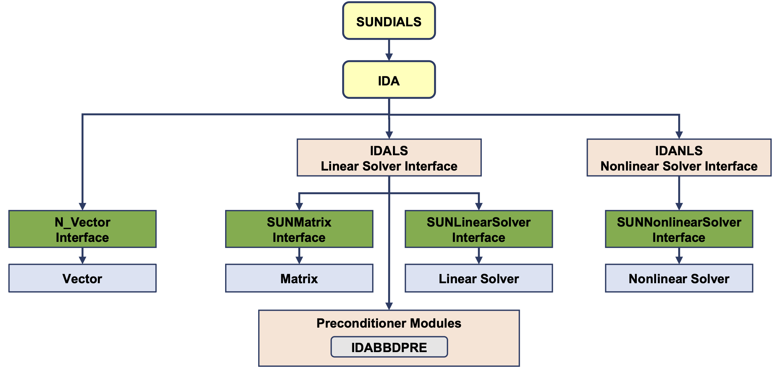
Fig. 5.1 Overall structure diagram of the IDA package. Components specific to IDA begin with “IDA” (IDALS, IDANLS, and IDABBDPRE), all other items correspond to generic SUNDIALS vector, matrix, and solver interfaces.
The overall organization of the IDA package is shown in
Fig. 5.1. IDA utilizes generic linear and nonlinear
solvers defined by the SUNLinearSolver (see §10) and
SUNNonlinearSolver interfaces (see §11) respectively. As
such, IDA has no knowledge of the method being used to solve the linear and
nonlinear systems that arise. For any given user problem, there exists a single
nonlinear solver interface and, if necessary, one of the linear system solver
interfaces is specified, and invoked as needed during the integration.
IDA has a single unified linear solver interface, IDALS, supporting both direct
and iterative linear solvers built using the generic SUNLinearSolver
interface (see §10). These solvers may utilize a SUNMatrix
object (see §9) for storing Jacobian information, or they may
be matrix-free. Since IDA can operate on any valid SUNLinearSolver, the set
of linear solver modules available to IDA will expand as new SUNLinearSolver
implementations are developed.
For users employing SUNMATRIX_DENSE or SUNMATRIX_BAND Jacobian matrices, IDA includes algorithms for their approximation through difference quotients, although the user also has the option of supplying a routine to compute the Jacobian (or an approximation to it) directly. This user-supplied routine is required when using sparse or user-supplied Jacobian matrices.
For users employing matrix-free iterative linear solvers, IDA includes an algorithm for the approximation by difference quotients of the product \(Jv\). Again, the user has the option of providing routines for this operation, in two phases: setup (preprocessing of Jacobian data) and multiplication.
For preconditioned iterative methods, the preconditioning must be supplied by the user, again in two phases: setup and solve. While there is no default choice of preconditioner analogous to the difference-quotient approximation in the direct case, the references [26, 31], together with the example and demonstration programs included with IDA, offer considerable assistance in building preconditioners.
IDA’s linear solver interface consists of four primary phases, devoted to (1) memory allocation and initialization, (2) setup of the matrix data involved, (3) solution of the system, and (4) freeing of memory. The setup and solution phases are separate because the evaluation of Jacobians and preconditioners is done only periodically during the integration, and only as required to achieve convergence. The call list within the central IDA module to each of the four associated functions is fixed, thus allowing the central module to be completely independent of the linear system method.
IDA also provides a preconditioner module, for use with any of the Krylov iterative linear solvers. It works in conjunction with the NVECTOR_PARALLEL and generates a preconditioner that is a block-diagonal matrix with each block being a banded matrix.
All state information used by IDA to solve a given problem is stored in
N_Vector instances. There is no global data in the IDA package, and so, in
this respect, it is reentrant. State information specific to the linear and
nonlinear solver are saved in the SUNLinearSolver and SUNNonlinearSolver
instances respectively. The reentrancy of IDA enables the setting where two or
more problems are solved by intermixed or parallel calls to different instances
of the package from within a single user program.