6.2. Mathematical Considerations
IDAS solves the initial-value problem (IVP) for a DAE system of the general form
where \(y\), \(\dot{y}\), and \(F\) are vectors in \(\mathbb{R}^N\), \(t\) is the independent variable, \(\dot{y} = \mathrm dy/\mathrm dt\), and initial values \(y_0\), \(\dot{y}_0\) are given. Often \(t\) is time, but it certainly need not be.
Additionally, if (6.1) depends on some parameters \(p \in \mathbb{R}^{N_p}\), i.e.
IDAS can also compute first order derivative information, performing either forward sensitivity analysis or adjoint sensitivity analysis. In the first case, IDAS computes the sensitivities of the solution with respect to the parameters \(p\), while in the second case, IDAS computes the gradient of a derived function with respect to the parameters \(p\).
6.2.1. Initial Condition
Prior to integrating a DAE initial-value problem, an important requirement is that the pair of vectors \(y_0\) and \(\dot{y}_0\) are both initialized to satisfy the DAE residual \(F(t_0,y_0, \dot{y}_0) = 0\). For a class of problems that includes so-called semi-explicit index-one systems, IDAS provides a routine that computes consistent initial conditions from a user’s initial guess [28]. For this, the user must identify sub-vectors of \(y\) (not necessarily contiguous), denoted \(y_d\) and \(y_a\), which are its differential and algebraic parts, respectively, such that \(F\) depends on \(\dot{y}_d\) but not on any components of \(\dot{y}_a\). The assumption that the system is “index one” means that for a given \(t\) and \(y_d\), the system \(F(t,y,\dot{y}) = 0\) defines \(y_a\) uniquely. In this case, a solver within IDAS computes \(y_a\) and \(\dot{y}_d\) at \(t = t_0\), given \(y_d\) and an initial guess for \(y_a\). A second available option with this solver also computes all of \(y(t_0)\) given \(\dot{y}(t_0)\); this is intended mainly for quasi-steady-state problems, where \(\dot{y}(t_0) = 0\) is given. In both cases, IDAS solves the system \(F(t_0,y_0, \dot{y}_0) = 0\) for the unknown components of \(y_0\) and \(\dot{y}_0\), using a Newton iteration augmented with a line search globalization strategy. In doing this, it makes use of the existing machinery that is to be used for solving the linear systems during the integration, in combination with certain tricks involving the step size (which is set artificially for this calculation). For problems that do not fall into either of these categories, the user is responsible for passing consistent values, or risks failure in the numerical integration.
6.2.2. IVP solution
The integration method used in IDAS is the variable-order, variable-coefficient BDF (Backward Differentiation Formula), in fixed-leading-coefficient form [23]. The method order ranges from 1 to 5, with the BDF of order \(q\) given by the multistep formula
where \(y_n\) and \(\dot{y}_n\) are the computed approximations to \(y(t_n)\) and \(\dot{y}(t_n)\), respectively, and the step size is \(h_n = t_n - t_{n-1}\). The coefficients \(\alpha_{n,i}\) are uniquely determined by the order \(q\), and the history of the step sizes. The application of the BDF (6.3) to the DAE system (6.1) results in a nonlinear algebraic system to be solved at each step:
In the process of controlling errors at various levels, IDAS uses a weighted root-mean-square norm, denoted \(\|\cdot\|_{\text{WRMS}}\), for all error-like quantities. The multiplicative weights used are based on the current solution and on the relative and absolute tolerances input by the user, namely
Because \(1/W_i\) represents a tolerance in the component \(y_i\), a vector whose norm is 1 is regarded as “small.” For brevity, we will usually drop the subscript WRMS on norms in what follows.
6.2.2.1. Nonlinear Solve
By default IDAS solves (6.4) with a Newton iteration but IDAS also allows for user-defined nonlinear solvers (see Chapter §11). Each Newton iteration requires the solution of a linear system of the form
where \(y_{n(m)}\) is the \(m\)-th approximation to \(y_n\). Here \(J\) is some approximation to the system Jacobian
where \(\alpha = \alpha_{n,0}/h_n\). The scalar \(\alpha\) changes whenever the step size or method order changes.
For the solution of the linear systems within the Newton iteration, IDAS provides several choices, including the option of a user-supplied linear solver (see Chapter §10). The linear solvers distributed with SUNDIALS are organized in two families, a direct family comprising direct linear solvers for dense, banded, or sparse matrices and a spils family comprising scaled preconditioned iterative (Krylov) linear solvers. The methods offered through these modules are as follows:
dense direct solvers, including an internal implementation, an interface to BLAS/LAPACK, an interface to MAGMA [158] and an interface to the oneMKL library [3],
band direct solvers, including an internal implementation or an interface to BLAS/LAPACK,
sparse direct solver interfaces to various libraries, including KLU [4, 45], SuperLU_MT [9, 47, 105], SuperLU_Dist [8, 70, 106, 107], and cuSPARSE [7],
SPGMR, a scaled preconditioned GMRES (Generalized Minimal Residual method) solver with or without restarts,
SPFGMR, a scaled preconditioned FGMRES (Flexible Generalized Minimal Residual method) solver with or without restarts,
SPBCG, a scaled preconditioned Bi-CGStab (Bi-Conjugate Gradient Stable method) solver,
SPTFQMR, a scaled preconditioned TFQMR (Transpose-Free Quasi-Minimal Residual method) solver, or
PCG, a scaled preconditioned CG (Conjugate Gradient method) solver.
For large stiff systems, where direct methods are not feasible, the combination of a BDF integrator and a preconditioned Krylov method yields a powerful tool because it combines established methods for stiff integration, nonlinear iteration, and Krylov (linear) iteration with a problem-specific treatment of the dominant source of stiffness, in the form of the user-supplied preconditioner matrix [26]. For the spils linear solvers with IDAS, preconditioning is allowed only on the left (see §6.2.3). Note that the dense, band, and sparse direct linear solvers can only be used with serial and threaded vector representations.
In the case of a matrix-based linear solver, the default Newton iteration is a Modified Newton iteration, in that the Jacobian \(J\) is fixed (and usually out of date) throughout the nonlinear iterations, with a coefficient \(\bar\alpha\) in place of \(\alpha\) in \(J\). However, in the case that a matrix-free iterative linear solver is used, the default Newton iteration is an Inexact Newton iteration, in which \(J\) is applied in a matrix-free manner, with matrix-vector products \(Jv\) obtained by either difference quotients or a user-supplied routine. In this case, the linear residual \(J\Delta y + G\) is nonzero but controlled. With the default Newton iteration, the matrix \(J\) and preconditioner matrix \(P\) are updated as infrequently as possible to balance the high costs of matrix operations against other costs. Specifically, this matrix update occurs when:
starting the problem,
the value \(\bar\alpha\) at the last update is such that \(\alpha / {\bar\alpha} < 3/5\) or \(\alpha / {\bar\alpha} > 5/3\), or
a non-fatal convergence failure occurred with an out-of-date \(J\) or \(P\).
The above strategy balances the high cost of frequent matrix evaluations and preprocessing with the slow convergence due to infrequent updates. To reduce storage costs on an update, Jacobian information is always reevaluated from scratch.
The default stopping test for nonlinear solver iterations in IDAS ensures that the iteration error \(y_n - y_{n(m)}\) is small relative to \(y\) itself. For this, we estimate the linear convergence rate at all iterations \(m>1\) as
where the \(\delta_m = y_{n(m)} - y_{n(m-1)}\) is the correction at iteration \(m=1,2,\ldots\). The nonlinear solver iteration is halted if \(R>0.9\). The convergence test at the \(m\)-th iteration is then
where \(S = R/(R-1)\) whenever \(m>1\) and \(R\le 0.9\). The user has the option of changing the constant in the convergence test from its default value of \(0.33\). The quantity \(S\) is set to \(S=20\) initially and whenever \(J\) or \(P\) is updated, and it is reset to \(S=100\) on a step with \(\alpha \neq \bar\alpha\). Note that at \(m=1\), the convergence test (6.8) uses an old value for \(S\). Therefore, at the first nonlinear solver iteration, we make an additional test and stop the iteration if \(\|\delta_1\| < 0.33 \cdot 10^{-4}\) (since such a \(\delta_1\) is probably just noise and therefore not appropriate for use in evaluating \(R\)). We allow only a small number (default value 4) of nonlinear iterations. If convergence fails with \(J\) or \(P\) current, we are forced to reduce the step size \(h_n\), and we replace \(h_n\) by \(h_n \eta_{\mathrm{cf}}\) (by default \(\eta_{\mathrm{cf}} = 0.25\)). The integration is halted after a preset number (default value 10) of convergence failures. Both the maximum number of allowable nonlinear iterations and the maximum number of nonlinear convergence failures can be changed by the user from their default values.
When an iterative method is used to solve the linear system, to minimize the effect of linear iteration errors on the nonlinear and local integration error controls, we require the preconditioned linear residual to be small relative to the allowed error in the nonlinear iteration, i.e., \(\| P^{-1}(Jx+G) \| < 0.05 \cdot 0.33\). The safety factor \(0.05\) can be changed by the user.
When the Jacobian is stored using either the SUNMATRIX_DENSE or SUNMATRIX_BAND matrix objects, the Jacobian \(J\) defined in (6.7) can be either supplied by the user or IDAS can compute \(J\) internally by difference quotients. In the latter case, we use the approximation
where \(U\) is the unit roundoff, \(h\) is the current step size, and \(W_j\) is the error weight for the component \(y_j\) defined by (6.5). We note that with sparse and user-supplied matrix objects, the Jacobian must be supplied by a user routine.
In the case of an iterative linear solver, if a routine for \(Jv\) is not supplied, such products are approximated by
where the increment \(\sigma = 1/\|v\|\). As an option, the user can specify a constant factor that is inserted into this expression for \(\sigma\).
6.2.2.2. Local Error Test
During the course of integrating the system, IDAS computes an estimate of the local truncation error, LTE, at the \(n\)-th time step, and requires this to satisfy the inequality
Asymptotically, LTE varies as \(h^{q+1}\) at step size \(h\) and order \(q\), as does the predictor-corrector difference \(\Delta_n \equiv y_n-y_{n(0)}\). Thus there is a constant \(C\) such that
and so the norm of LTE is estimated as \(|C| \cdot \|\Delta_n\|\). In addition, IDAS requires that the error in the associated polynomial interpolant over the current step be bounded by 1 in norm. The leading term of the norm of this error is bounded by \(\bar{C} \|\Delta_n\|\) for another constant \(\bar{C}\). Thus the local error test in IDAS is
A user option is available by which the algebraic components of the error vector are omitted from the test (6.9), if these have been so identified.
6.2.2.3. Step Size and Order Selection
In IDAS, the local error test is tightly coupled with the logic for selecting the step size and order. First, there is an initial phase that is treated specially; for the first few steps, the step size is doubled and the order raised (from its initial value of 1) on every step, until (a) the local error test (6.9) fails, (b) the order is reduced (by the rules given below), or (c) the order reaches 5 (the maximum). For step and order selection on the general step, IDAS uses a different set of local error estimates, based on the asymptotic behavior of the local error in the case of fixed step sizes. At each of the orders \(q'\) equal to \(q\), \(q-1\) (if \(q > 1\)), \(q-2\) (if \(q > 2\)), or \(q+1\) (if \(q < 5\)), there are constants \(C(q')\) such that the norm of the local truncation error at order \(q'\) satisfies
where \(\phi(k)\) is a modified divided difference of order \(k\) that is retained by IDAS (and behaves asymptotically as \(h^k\)). Thus the local truncation errors are estimated as ELTE\((q') = C(q')\|\phi(q'+1)\|\) to select step sizes. But the choice of order in IDAS is based on the requirement that the scaled derivative norms, \(\|h^k y^{(k)}\|\), are monotonically decreasing with \(k\), for \(k\) near \(q\). These norms are again estimated using the \(\phi(k)\), and in fact
The step/order selection begins with a test for monotonicity that is made even before the local error test is performed. Namely, the order is reset to \(q' = q-1\) if (a) \(q=2\) and \(T(1)\leq T(2)/2\), or (b) \(q > 2\) and \(\max\{T(q-1),T(q-2)\} \leq T(q)\); otherwise \(q' = q\). Next the local error test (6.9) is performed, and if it fails, the step is redone at order \(q\leftarrow q'\) and a new step size \(h'\). The latter is based on the \(h^{q+1}\) asymptotic behavior of \(\text{ELTE}(q)\), and, with safety factors, is given by
The value of \(\eta\) is adjusted so that \(\eta_{\mathrm{min\_ef}} \leq \eta \leq \eta_{\mathrm{low}}\) (by default \(\eta_{\mathrm{min\_ef}} = 0.25\) and \(\eta_{\mathrm{low}} = 0.9\)) before setting \(h \leftarrow h' = \eta h\). If the local error test fails a second time, IDA uses \(\eta = \eta_{\mathrm{min\_ef}}\), and on the third and subsequent failures it uses \(q = 1\) and \(\eta = \eta_{\mathrm{min\_ef}}\). After 10 failures, IDA returns with a give-up message.
As soon as the local error test has passed, the step and order for the next step may be adjusted. No order change is made if \(q' = q-1\) from the prior test, if \(q = 5\), or if \(q\) was increased on the previous step. Otherwise, if the last \(q+1\) steps were taken at a constant order \(q < 5\) and a constant step size, IDAS considers raising the order to \(q+1\). The logic is as follows:
If \(q = 1\), then set \(q = 2\) if \(T(2) < T(1)/2\).
If \(q > 1\) then
set \(q \leftarrow q-1\) if \(T(q-1) \leq \min\{T(q),T(q+1)\}\), else
set \(q \leftarrow q+1\) if \(T(q+1) < T(q)\), otherwise
leave \(q\) unchanged, in this case \(T(q-1) > T(q) \leq T(q+1)\)
In any case, the new step size \(h'\) is set much as before:
The value of \(\eta\) is adjusted such that
If \(\eta_{\mathrm{min\_fx}} < \eta < \eta_{\mathrm{max\_fx}}\), set \(\eta = 1\). The defaults are \(\eta_{\mathrm{min\_fx}} = 1\) and \(\eta_{\mathrm{max\_fx}} = 2\).
If \(\eta \geq \eta_{\mathrm{max\_fx}}\), the step size growth is restricted to \(\eta_{\mathrm{max\_fx}} \leq \eta \leq \eta_{\mathrm{max}}\) with \(\eta_{\mathrm{max}} = 2\) by default.
If \(\eta \leq \eta_{\mathrm{min\_fx}}\), the step size reduction is restricted to \(\eta_{\mathrm{min}} \leq \eta \leq \eta_{\mathrm{low}}\) with \(\eta_{\mathrm{min}} = 0.5\) and \(\eta_{\mathrm{low}} = 0.9\) by default.
Thus we do not increase the step size unless it can be doubled. If a step size reduction is called for, the step size will be cut by at least 10% and up to 50% for the next step. See [23] for details.
Finally \(h\) is set to \(h' = \eta h\) and \(|h|\) is restricted to \(h_{\text{min}} \leq |h| \leq h_{\text{max}}\) with the defaults \(h_{\text{min}} = 0.0\) and \(h_{\text{max}} = \infty\).
Normally, IDAS takes steps until a user-defined output value \(t = t_{\text{out}}\) is overtaken, and then computes \(y(t_{\text{out}})\) by interpolation. However, a “one step” mode option is available, where control returns to the calling program after each step. There are also options to force IDAS not to integrate past a given stopping point \(t = t_{\text{stop}}\).
6.2.2.4. Inequality Constraints
IDAS permits the user to impose optional inequality constraints on individual components of the solution vector \(y\). Any of the following four constraints can be imposed: \(y_i > 0\), \(y_i < 0\), \(y_i \geq 0\), or \(y_i \leq 0\). The constraint satisfaction is tested after a successful nonlinear system solution. If any constraint fails, we declare a convergence failure of the nonlinear iteration and reduce the step size. Rather than cutting the step size by some arbitrary factor, IDAS estimates a new step size \(h'\) using a linear approximation of the components in \(y\) that failed the constraint test (including a safety factor of \(0.9\) to cover the strict inequality case). These additional constraints are also imposed during the calculation of consistent initial conditions. If a step fails to satisfy the constraints repeatedly within a step attempt then the integration is halted and an error is returned. In this case the user may need to employ other strategies as discussed in §6.4.1.3.2 to satisfy the inequality constraints.
6.2.3. Preconditioning
When using a nonlinear solver that requires the solution of a linear system of the form \(J \Delta y = - G\) (e.g., the default Newton iteration), IDAS makes repeated use of a linear solver. If this linear system solve is done with one of the scaled preconditioned iterative linear solvers supplied with SUNDIALS, these solvers are rarely successful if used without preconditioning; it is generally necessary to precondition the system in order to obtain acceptable efficiency. A system \(A x = b\) can be preconditioned on the left, on the right, or on both sides. The Krylov method is then applied to a system with the matrix \(P^{-1}A\), or \(AP^{-1}\), or \(P_L^{-1} A P_R^{-1}\), instead of \(A\). However, within IDAS, preconditioning is allowed only on the left, so that the iterative method is applied to systems \((P^{-1}J)\Delta y = -P^{-1}G\). Left preconditioning is required to make the norm of the linear residual in the nonlinear iteration meaningful; in general, \(\| J \Delta y + G \|\) is meaningless, since the weights used in the WRMS-norm correspond to \(y\).
In order to improve the convergence of the Krylov iteration, the preconditioner matrix \(P\) should in some sense approximate the system matrix \(A\). Yet at the same time, in order to be cost-effective, the matrix \(P\) should be reasonably efficient to evaluate and solve. Finding a good point in this tradeoff between rapid convergence and low cost can be very difficult. Good choices are often problem-dependent (for example, see [26] for an extensive study of preconditioners for reaction-transport systems).
Typical preconditioners used with IDAS are based on approximations to the iteration matrix of the systems involved; in other words, \(P \approx \dfrac{\partial F}{\partial y} + \alpha\dfrac{\partial F}{\partial \dot{y}}\), where \(\alpha\) is a scalar inversely proportional to the integration step size \(h\). Because the Krylov iteration occurs within a nonlinear solver iteration and further also within a time integration, and since each of these iterations has its own test for convergence, the preconditioner may use a very crude approximation, as long as it captures the dominant numerical feature(s) of the system. We have found that the combination of a preconditioner with the Newton-Krylov iteration, using even a fairly poor approximation to the Jacobian, can be surprisingly superior to using the same matrix without Krylov acceleration (i.e., a modified Newton iteration), as well as to using the Newton-Krylov method with no preconditioning.
6.2.4. Rootfinding
The IDAS solver has been augmented to include a rootfinding feature. This means that, while integratnuming the Initial Value Problem (6.1), IDAS can also find the roots of a set of user-defined functions \(g_i(t,y,\dot{y})\) that depend on \(t\), the solution vector \(y = y(t)\), and its \(t-\)derivative \(\dot{y}(t)\). The number of these root functions is arbitrary, and if more than one \(g_i\) is found to have a root in any given interval, the various root locations are found and reported in the order that they occur on the \(t\) axis, in the direction of integration.
Generally, this rootfinding feature finds only roots of odd multiplicity, corresponding to changes in sign of \(g_i(t,y(t),\dot{y}(t))\), denoted \(g_i(t)\) for short. If a user root function has a root of even multiplicity (no sign change), it will probably be missed by IDAS. If such a root is desired, the user should reformulate the root function so that it changes sign at the desired root.
The basic scheme used is to check for sign changes of any \(g_i(t)\) over each time step taken, and then (when a sign change is found) to home in on the root (or roots) with a modified secant method [79]. In addition, each time \(g\) is computed, IDAS checks to see if \(g_i(t) = 0\) exactly, and if so it reports this as a root. However, if an exact zero of any \(g_i\) is found at a point \(t\), IDAS computes \(g\) at \(t + \delta\) for a small increment \(\delta\), slightly further in the direction of integration, and if any \(g_i(t + \delta)=0\) also, IDAS stops and reports an error. This way, each time IDAS takes a time step, it is guaranteed that the values of all \(g_i\) are nonzero at some past value of \(t\), beyond which a search for roots is to be done.
At any given time in the course of the time-stepping, after suitable checking and adjusting has been done, IDAS has an interval \((t_{lo},t_{hi}]\) in which roots of the \(g_i(t)\) are to be sought, such that \(t_{hi}\) is further ahead in the direction of integration, and all \(g_i(t_{lo}) \neq 0\). The endpoint \(t_{hi}\) is either \(t_n\), the end of the time step last taken, or the next requested output time \(t_{\text{out}}\) if this comes sooner. The endpoint \(t_{lo}\) is either \(t_{n-1}\), or the last output time \(t_{\text{out}}\) (if this occurred within the last step), or the last root location (if a root was just located within this step), possibly adjusted slightly toward \(t_n\) if an exact zero was found. The algorithm checks \(g\) at \(t_{hi}\) for zeros and for sign changes in \((t_{lo},t_{hi})\). If no sign changes are found, then either a root is reported (if some \(g_i(t_{hi}) = 0\)) or we proceed to the next time interval (starting at \(t_{hi}\)). If one or more sign changes were found, then a loop is entered to locate the root to within a rather tight tolerance, given by
Whenever sign changes are seen in two or more root functions, the one deemed most likely to have its root occur first is the one with the largest value of \(|g_i(t_{hi})|/|g_i(t_{hi}) - g_i(t_{lo})|\), corresponding to the closest to \(t_{lo}\) of the secant method values. At each pass through the loop, a new value \(t_{mid}\) is set, strictly within the search interval, and the values of \(g_i(t_{mid})\) are checked. Then either \(t_{lo}\) or \(t_{hi}\) is reset to \(t_{mid}\) according to which subinterval is found to have the sign change. If there is none in \((t_{lo},t_{mid})\) but some \(g_i(t_{mid}) = 0\), then that root is reported. The loop continues until \(|t_{hi}-t_{lo}| < \tau\), and then the reported root location is \(t_{hi}\).
In the loop to locate the root of \(g_i(t)\), the formula for \(t_{mid}\) is
where \(\alpha\) a weight parameter. On the first two passes through the loop, \(\alpha\) is set to \(1\), making \(t_{mid}\) the secant method value. Thereafter, \(\alpha\) is reset according to the side of the subinterval (low vs high, i.e. toward \(t_{lo}\) vs toward \(t_{hi}\)) in which the sign change was found in the previous two passes. If the two sides were opposite, \(\alpha\) is set to 1. If the two sides were the same, \(\alpha\) is halved (if on the low side) or doubled (if on the high side). The value of \(t_{mid}\) is closer to \(t_{lo}\) when \(\alpha < 1\) and closer to \(t_{hi}\) when \(\alpha > 1\). If the above value of \(t_{mid}\) is within \(\tau/2\) of \(t_{lo}\) or \(t_{hi}\), it is adjusted inward, such that its fractional distance from the endpoint (relative to the interval size) is between 0.1 and 0.5 (0.5 being the midpoint), and the actual distance from the endpoint is at least \(\tau/2\).
6.2.5. Pure quadrature integration
In many applications, and most notably during the backward integration phase of an adjoint sensitivity analysis run §6.2.7 it is of interest to compute integral quantities of the form
The most effective approach to compute \(z(t)\) is to extend the original problem with the additional ODEs (obtained by applying Leibnitz’s differentiation rule):
Note that this is equivalent to using a quadrature method based on the underlying linear multistep polynomial representation for \(y(t)\).
This can be done at the “user level” by simply exposing to IDAS the extended DAE system (6.2) + (6.10). However, in the context of an implicit integration solver, this approach is not desirable since the nonlinear solver module will require the Jacobian (or Jacobian-vector product) of this extended DAE. Moreover, since the additional states, \(z\), do not enter the right-hand side of the ODE (6.10) and therefore the residual of the extended DAE system does not depend on \(z\), it is much more efficient to treat the ODE system (6.10) separately from the original DAE system (6.2) by “taking out” the additional states \(z\) from the nonlinear system (6.4) that must be solved in the correction step of the LMM. Instead, “corrected” values \(z_n\) are computed explicitly as
once the new approximation \(y_n\) is available.
The quadrature variables \(z\) can be optionally included in the error test, in which case corresponding relative and absolute tolerances must be provided.
6.2.6. Forward sensitivity analysis
Typically, the governing equations of complex, large-scale models depend on various parameters, through the right-hand side vector and/or through the vector of initial conditions, as in (6.2). In addition to numerically solving the DAEs, it may be desirable to determine the sensitivity of the results with respect to the model parameters. Such sensitivity information can be used to estimate which parameters are most influential in affecting the behavior of the simulation or to evaluate optimization gradients (in the setting of dynamic optimization, parameter estimation, optimal control, etc.).
The solution sensitivity with respect to the model parameter \(p_i\) is defined as the vector \(s_i (t) = {\partial y(t)}/{\partial p_i}\) and satisfies the following forward sensitivity equations (or sensitivity equations for short):
obtained by applying the chain rule of differentiation to the original DAEs (6.2).
When performing forward sensitivity analysis, IDAS carries out the time integration of the combined system, (6.2) and (6.11), by viewing it as a DAE system of size \(N(N_s+1)\), where \(N_s\) is the number of model parameters \(p_i\), with respect to which sensitivities are desired (\(N_s \le N_p\)). However, major improvements in efficiency can be made by taking advantage of the special form of the sensitivity equations as linearizations of the original DAEs. In particular, the original DAE system and all sensitivity systems share the same Jacobian matrix \(J\) in (6.7).
The sensitivity equations are solved with the same linear multistep formula that was selected for the original DAEs and the same linear solver is used in the correction phase for both state and sensitivity variables. In addition, IDAS offers the option of including (full error control) or excluding (partial error control) the sensitivity variables from the local error test.
6.2.6.1. Forward sensitivity methods
In what follows we briefly describe three methods that have been proposed for the solution of the combined DAE and sensitivity system for the vector \({\hat y} = [y, s_1, \ldots , s_{N_s}]\).
Staggered Direct In this approach [37], the nonlinear system (6.4) is first solved and, once an acceptable numerical solution is obtained, the sensitivity variables at the new step are found by directly solving (6.11) after the BDF discretization is used to eliminate \({\dot s}_i\). Although the system matrix of the above linear system is based on exactly the same information as the matrix \(J\) in (6.7), it must be updated and factored at every step of the integration, in contrast to an evaluation of \(J\) which is updated only occasionally. For problems with many parameters (relative to the problem size), the staggered direct method can outperform the methods described below [104]. However, the computational cost associated with matrix updates and factorizations makes this method unattractive for problems with many more states than parameters (such as those arising from semidiscretization of PDEs) and is therefore not implemented in IDAS.
Simultaneous Corrector In this method [110], the discretization is applied simultaneously to both the original equations (6.2) and the sensitivity systems (6.11) resulting in an “extended” nonlinear system \({\hat G}({\hat y}_n) = 0\) where \({\hat y_n} = [ y_n, \ldots, s_i, \ldots ]\). This combined nonlinear system can be solved using a modified Newton method as in (6.6) by solving the corrector equation
(6.12)\[{\hat J}[{\hat y}_{n(m+1)}-{\hat y}_{n(m)}]=-{\hat G}({\hat y}_{n(m)})\]at each iteration, where
\[\begin{split}{\hat J} = \begin{bmatrix} J & & & & \\ J_1 & J & & & \\ J_2 & 0 & J & & \\ \vdots & \vdots & \ddots & \ddots & \\ J_{N_s} & 0 & \ldots & 0 & J \end{bmatrix} \, ,\end{split}\]\(J\) is defined as in (6.7), and \(J_i = ({\partial}/{\partial y})\left[ F_y s_i + F_{\dot y} {\dot s_i} + F_{p_i} \right]\). It can be shown that 2-step quadratic convergence can be retained by using only the block-diagonal portion of \({\hat J}\) in the corrector equation (6.12). This results in a decoupling that allows the reuse of \(J\) without additional matrix factorizations. However, the sum \(F_y s_i + F_{\dot y} {\dot s_i} + F_{p_i}\) must still be reevaluated at each step of the iterative process (6.12) to update the sensitivity portions of the residual \({\hat G}\).
Staggered corrector In this approach [59], as in the staggered direct method, the nonlinear system (6.4) is solved first using the Newton iteration (6.6). Then, for each sensitivity vector \(\xi \equiv s_i\), a separate Newton iteration is used to solve the sensitivity system (6.11):
(6.13)\[\begin{split}\begin{gathered} J [\xi_{n(m+1)} - \xi_{n(m)}]= \\ - \left[ F_y (t_n, y_n, \dot y_n) \xi_{n(m)} + F_{\dot y} (t_n, y_n, \dot y_n) \cdot h_n^{-1} \left( \alpha_{n,0} \xi_{n(m)} + \sum_{i=1}^q \alpha_{n,i} \xi_{n-i} \right) + F_{p_i} (t_n, y_n, \dot y_n) \right] \, . \end{gathered}\end{split}\]In other words, a modified Newton iteration is used to solve a linear system. In this approach, the matrices \(\partial F / \partial y\), \(\partial F / \partial \dot y\) and vectors \(\partial f / \partial p_i\) need be updated only once per integration step, after the state correction phase (6.6) has converged.
IDAS implements both the simultaneous corrector method and the staggered corrector method.
An important observation is that the staggered corrector method, combined with a Krylov linear solver, effectively results in a staggered direct method. Indeed, the Krylov solver requires only the action of the matrix \(J\) on a vector, and this can be provided with the current Jacobian information. Therefore, the modified Newton procedure (6.13) will theoretically converge after one iteration.
6.2.6.2. Selection of the absolute tolerances for sensitivity variables
If the sensitivities are included in the error test, IDAS provides an automated estimation of absolute tolerances for the sensitivity variables based on the absolute tolerance for the corresponding state variable. The relative tolerance for sensitivity variables is set to be the same as for the state variables. The selection of absolute tolerances for the sensitivity variables is based on the observation that the sensitivity vector \(s_i\) will have units of \([y]/[p_i]\). With this, the absolute tolerance for the \(j\)-th component of the sensitivity vector \(s_i\) is set to \({\mbox{atol}_j}/{|{\bar p}_i|}\), where \(\mbox{atol}_j\) are the absolute tolerances for the state variables and \(\bar p\) is a vector of scaling factors that are dimensionally consistent with the model parameters \(p\) and give an indication of their order of magnitude. This choice of relative and absolute tolerances is equivalent to requiring that the weighted root-mean-square norm of the sensitivity vector \(s_i\) with weights based on \(s_i\) be the same as the weighted root-mean-square norm of the vector of scaled sensitivities \({\bar s}_i = |{\bar p}_i| s_i\) with weights based on the state variables (the scaled sensitivities \({\bar s}_i\) being dimensionally consistent with the state variables). However, this choice of tolerances for the \(s_i\) may be a poor one, and the user of IDAS can provide different values as an option.
6.2.6.3. Evaluation of the sensitivity right-hand side
There are several methods for evaluating the residual functions in the sensitivity systems (6.11): analytic evaluation, automatic differentiation, complex-step approximation, and finite differences (or directional derivatives). IDAS provides all the software hooks for implementing interfaces to automatic differentiation (AD) or complex-step approximation; future versions will include a generic interface to AD-generated functions. At the present time, besides the option for analytical sensitivity right-hand sides (user-provided), IDAS can evaluate these quantities using various finite difference-based approximations to evaluate the terms \((\partial F / \partial y) s_i + (\partial F / \partial \dot y) \dot s_i\) and \((\partial f / \partial p_i)\), or using directional derivatives to evaluate \(\left[ (\partial F / \partial y) s_i + (\partial F / \partial \dot y) \dot s_i + (\partial f / \partial p_i) \right]\). As is typical for finite differences, the proper choice of perturbations is a delicate matter. IDAS takes into account several problem-related features: the relative DAE error tolerance \(\mbox{rtol}\), the machine unit roundoff \(U\), the scale factor \({\bar p}_i\), and the weighted root-mean-square norm of the sensitivity vector \(s_i\).
Using central finite differences as an example, the two terms \((\partial F / \partial y) s_i + (\partial F / \partial \dot y) \dot s_i\) and \(\partial f / \partial p_i\) in (6.11) can be evaluated either separately:
or simultaneously:
or by adaptively switching between (6.14) + (6.15) and (6.16), depending on the relative size of the two finite difference increments \(\sigma_i\) and \(\sigma_y\). In the adaptive scheme, if \(\rho = \max(\sigma_i/\sigma_y,\sigma_y/\sigma_i)\), we use separate evaluations if \(\rho > \rho_{max}\) (an input value), and simultaneous evaluations otherwise.
These procedures for choosing the perturbations (\(\sigma_i\), \(\sigma_y\), \(\sigma\)) and switching between derivative formulas have also been implemented for one-sided difference formulas. Forward finite differences can be applied to \((\partial F / \partial y) s_i + (\partial F / \partial \dot y) \dot s_i\) and \(\partial F / \partial p_i\) separately, or the single directional derivative formula
can be used. In IDAS, the default value of \(\rho_{max}=0\) indicates the use of the second-order centered directional derivative formula (6.16) exclusively. Otherwise, the magnitude of \(\rho_{max}\) and its sign (positive or negative) indicates whether this switching is done with regard to (centered or forward) finite differences, respectively.
6.2.6.4. Quadratures depending on forward sensitivities
If pure quadrature variables are also included in the problem definition (see §6.2.5), IDAS does not carry their sensitivities automatically. Instead, we provide a more general feature through which integrals depending on both the states \(y\) of (6.2) and the state sensitivities \(s_i\) of (6.11) can be evaluated. In other words, IDAS provides support for computing integrals of the form:
If the sensitivities of the quadrature variables \(z\) of (6.10) are desired, these can then be computed by using:
as integrands for \(\bar z\), where \(q_y\), \(q_{\dot{y}}\), and \(q_p\) are the partial derivatives of the integrand function \(q\) of (6.10).
As with the quadrature variables \(z\), the new variables \(\bar z\) are also excluded from any nonlinear solver phase and “corrected” values \(\bar z_n\) are obtained through explicit formulas.
6.2.7. Adjoint sensitivity analysis
In the forward sensitivity approach described in the previous section, obtaining sensitivities with respect to \(N_s\) parameters is roughly equivalent to solving an DAE system of size \((1+N_s) N\). This can become prohibitively expensive, especially for large-scale problems, if sensitivities with respect to many parameters are desired. In this situation, the adjoint sensitivity method is a very attractive alternative, provided that we do not need the solution sensitivities \(s_i\), but rather the gradients with respect to model parameters of a relatively few derived functionals of the solution. In other words, if \(y(t)\) is the solution of (6.2), we wish to evaluate the gradient \({\mathrm dG}/{\mathrm dp}\) of
or, alternatively, the gradient \({\mathrm dg}/{\mathrm dp}\) of the function \(g(t, y,p)\) at the final time \(t = T\). The function \(g\) must be smooth enough that \(\partial g / \partial y\) and \(\partial g / \partial p\) exist and are bounded.
In what follows, we only sketch the analysis for the sensitivity problem for both \(G\) and \(g\). For details on the derivation see [36].
6.2.7.1. Sensitivity of \(G(p)\)
We focus first on solving the sensitivity problem for \(G(p)\) defined by (6.17). Introducing a Lagrange multiplier \(\lambda\), we form the augmented objective function
Since \(F(t, y,\dot y, p)=0\), the sensitivity of \(G\) with respect to \(p\) is
where subscripts on functions such as \(F\) or \(g\) are used to denote partial derivatives. By integration by parts, we have
where \((\cdots)'\) denotes the \(t-\)derivative. Thus equation (6.18) becomes
Now by requiring \(\lambda\) to satisfy
we obtain
Note that \(y_p\) at \(t=t_0\) is the sensitivity of the initial conditions with respect to \(p\), which is easily obtained. To find the initial conditions (at \(t = T\)) for the adjoint system, we must take into consideration the structure of the DAE system.
For index-0 and index-1 DAE systems, we can simply take
yielding the sensitivity equation for \({dG}/{dp}\)
This choice will not suffice for a Hessenberg index-2 DAE system. For a derivation of proper final conditions in such cases, see [36].
The first thing to notice about the adjoint system (6.19) is that there is no explicit specification of the parameters \(p\); this implies that, once the solution \(\lambda\) is found, the formula (6.20) can then be used to find the gradient of \(G\) with respect to any of the parameters \(p\). The second important remark is that the adjoint system (6.19) is a terminal value problem which depends on the solution \(y(t)\) of the original IVP (6.2). Therefore, a procedure is needed for providing the states \(y\) obtained during a forward integration phase of (6.2) to IDAS during the backward integration phase of (6.19). The approach adopted in IDAS, based on checkpointing, is described in §6.2.7.3 below.
6.2.7.2. Sensitivity of \(g(T,p)\)
Now let us consider the computation of \({\mathrm dg}/{\mathrm dp}(T)\). From \({\mathrm dg}/{\mathrm dp}(T) = ({\mathrm d}/{\mathrm dT})({\mathrm dG}/{\mathrm dp})\) and equation (6.20), we have
where \(\lambda_T\) denotes \({\partial \lambda}/{\partial T}\). For index-0 and index-1 DAEs, we obtain
while for a Hessenberg index-2 DAE system we have
The corresponding adjoint equations are
For index-0 and index-1 DAEs (as shown above, the index-2 case is different), to find the boundary condition for this equation we write \(\lambda\) as \(\lambda(t, T)\) because it depends on both \(t\) and \(T\). Then
Taking the total derivative, we obtain
Since \(\lambda_t\) is just \(\dot \lambda\), we have the boundary condition
For the index-one DAE case, the above relation and (6.19) yield
For the regular implicit ODE case, \(F_{\dot{y}}\) is invertible; thus we have \(\lambda(T, T) = 0\), which leads to \(\lambda_T(T) = - \dot{\lambda}(T)\). As with the final conditions for \(\lambda(T)\) in (6.19), the above selection for \(\lambda_T(T)\) is not sufficient for index-two Hessenberg DAEs (see [36] for details).
6.2.7.3. Checkpointing scheme
During the backward integration, the evaluation of the right-hand side of the adjoint system requires, at the current time, the states \(y\) which were computed during the forward integration phase. Since IDAS implements variable-step integration formulas, it is unlikely that the states will be available at the desired time and so some form of interpolation is needed. The IDAS implementation being also variable-order, it is possible that during the forward integration phase the order may be reduced as low as first order, which means that there may be points in time where only \(y\) and \({\dot y}\) are available. These requirements therefore limit the choices for possible interpolation schemes. IDAS implements two interpolation methods: a cubic Hermite interpolation algorithm and a variable-degree polynomial interpolation method which attempts to mimic the BDF interpolant for the forward integration.
However, especially for large-scale problems and long integration intervals, the number and size of the vectors \(y\) and \({\dot y}\) that would need to be stored make this approach computationally intractable. Thus, IDAS settles for a compromise between storage space and execution time by implementing a so-called checkpointing scheme. At the cost of at most one additional forward integration, this approach offers the best possible estimate of memory requirements for adjoint sensitivity analysis. To begin with, based on the problem size \(N\) and the available memory, the user decides on the number \(N_d\) of data pairs (\(y\), \({\dot y}\)) if cubic Hermite interpolation is selected, or on the number \(N_d\) of \(y\) vectors in the case of variable-degree polynomial interpolation, that can be kept in memory for the purpose of interpolation. Then, during the first forward integration stage, after every \(N_d\) integration steps a checkpoint is formed by saving enough information (either in memory or on disk) to allow for a hot restart, that is a restart which will exactly reproduce the forward integration. In order to avoid storing Jacobian-related data at each checkpoint, a reevaluation of the iteration matrix is forced before each checkpoint. At the end of this stage, we are left with \(N_c\) checkpoints, including one at \(t_0\). During the backward integration stage, the adjoint variables are integrated backwards from \(T\) to \(t_0\), going from one checkpoint to the previous one. The backward integration from checkpoint \(i+1\) to checkpoint \(i\) is preceded by a forward integration from \(i\) to \(i+1\) during which the \(N_d\) vectors \(y\) (and, if necessary \({\dot y}\)) are generated and stored in memory for interpolation.
Note
The degree of the interpolation polynomial is always that of the current BDF order for the forward interpolation at the first point to the right of the time at which the interpolated value is sought (unless too close to the \(i\)-th checkpoint, in which case it uses the BDF order at the right-most relevant point). However, because of the FLC BDF implementation (see §6.2.2), the resulting interpolation polynomial is only an approximation to the underlying BDF interpolant.
The Hermite cubic interpolation option is present because it was implemented
chronologically first and it is also used by other adjoint solvers
(e.g. DASPKADJOINT). The variable-degree polynomial is more
memory-efficient (it requires only half of the memory storage of the cubic
Hermite interpolation) and is more accurate.
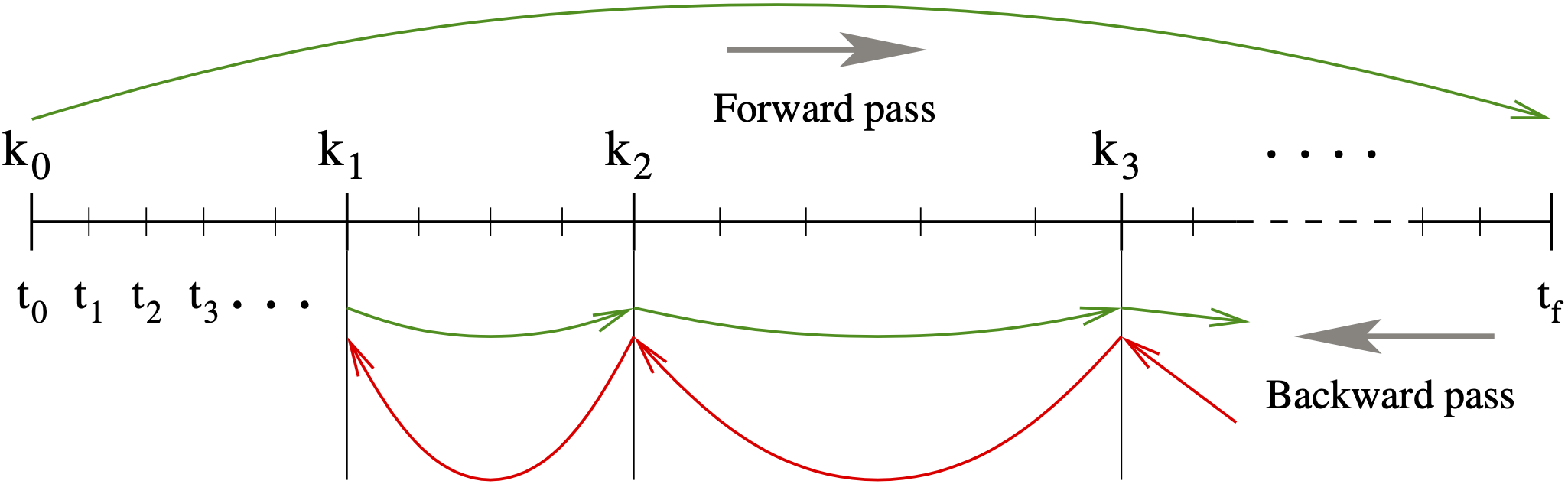
Fig. 6.1 Illustration of the checkpointing algorithm for generation of the forward solution during the integration of the adjoint system.
This approach transfers the uncertainty in the number of integration steps in the forward integration phase to uncertainty in the final number of checkpoints. However, \(N_c\) is much smaller than the number of steps taken during the forward integration, and there is no major penalty for writing/reading the checkpoint data to/from a temporary file. Note that, at the end of the first forward integration stage, interpolation data are available from the last checkpoint to the end of the interval of integration. If no checkpoints are necessary (\(N_d\) is larger than the number of integration steps taken in the solution of (6.2)), the total cost of an adjoint sensitivity computation can be as low as one forward plus one backward integration. In addition, IDAS provides the capability of reusing a set of checkpoints for multiple backward integrations, thus allowing for efficient computation of gradients of several functionals (6.17).
Finally, we note that the adjoint sensitivity module in IDAS provides the necessary infrastructure to integrate backwards in time any DAE terminal value problem dependent on the solution of the IVP (6.2), including adjoint systems (6.19) or (6.24), as well as any other quadrature ODEs that may be needed in evaluating the integrals in (6.20). In particular, for DAE systems arising from semi-discretization of time-dependent PDEs, this feature allows for integration of either the discretized adjoint PDE system or the adjoint of the discretized PDE.
6.2.8. Second-order sensitivity analysis
In some applications (e.g., dynamically-constrained optimization) it may be desirable to compute second-order derivative information. Considering the DAE problem (6.2) and some model output functional \(g(y)\), the Hessian \(\mathrm d^2g/\mathrm dp^2\) can be obtained in a forward sensitivity analysis setting as
where \(\otimes\) is the Kronecker product. The second-order sensitivities are solution of the matrix DAE system:
where \(y_p\) denotes the first-order sensitivity matrix, the solution of \(N_p\) systems (6.11), and \(y_{pp}\) is a third-order tensor. It is easy to see that, except for situations in which the number of parameters \(N_p\) is very small, the computational cost of this so-called forward-over-forward approach is exorbitant as it requires the solution of \(N_p + N_p^2\) additional DAE systems of the same dimension as (6.2).
Note
For the sake of simplifity in presentation, we do not include explicit dependencies of \(g\) on time \(t\) or parameters \(p\). Moreover, we only consider the case in which the dependency of the original DAE (6.2) on the parameters \(p\) is through its initial conditions only. For details on the derivation in the general case, see [115].
A much more efficient alternative is to compute Hessian-vector products using a so-called forward-over-adjoint approach. This method is based on using the same “trick” as the one used in computing gradients of pointwise functionals with the adjoint method, namely applying a formal directional forward derivation to the gradient of (6.20) (or the equivalent one for a pointwise functional \(g(T, y(T))\)). With that, the cost of computing a full Hessian is roughly equivalent to the cost of computing the gradient with forward sensitivity analysis. However, Hessian-vector products can be cheaply computed with one additional adjoint solve.
As an illustration, consider the ODE problem (the derivation for the general DAE case is too involved for the purposes of this discussion)
depending on some parameters \(p\) through the initial conditions only and consider the model functional output \(G(p) = \int_{t_0}^{t_f} g(t,y) \, \mathrm dt\). It can be shown that the product between the Hessian of \(G\) (with respect to the parameters \(p\)) and some vector \(u\) can be computed as
where \(\lambda\) and \(\mu\) are solutions of
In the above equation, \(s = y_p u\) is a linear combination of the columns of the sensitivity matrix \(y_p\). The forward-over-adjoint approach hinges crucially on the fact that \(s\) can be computed at the cost of a forward sensitivity analysis with respect to a single parameter (the last ODE problem above) which is possible due to the linearity of the forward sensitivity equations (6.11).
Therefore (and this is also valid for the DAE case), the cost of computing the Hessian-vector product is roughly that of two forward and two backward integrations of a system of DAEs of size \(N\). For more details, including the corresponding formulas for a pointwise model functional output, see the work by Ozyurt and Barton [115] who discuss this problem for ODE initial value problems. As far as we know, there is no published equivalent work on DAE problems. However, the derivations given in [115] for ODE problems can be extended to DAEs with some careful consideration given to the derivation of proper final conditions on the adjoint systems, following the ideas presented in [36].
To allow the foward-over-adjoint approach described above, IDAS provides support for:
the integration of multiple backward problems depending on the same underlying forward problem (6.2), and
the integration of backward problems and computation of backward quadratures depending on both the states \(y\) and forward sensitivities (for this particular application, \(s\)) of the original problem (6.2).